Table of Contents
- 5.0 Overview
- 5.1 Atmospheric Moisture
- 5.2 Adiabatic Processes and Vertical Distribution of Moisture
- 5.3 Precipitation
- 5.3.1 Precipitation Processes
- 5.3.2 The Impact of Aerosols: Maritime and Continental
- 5.3.3 Classification of Tropical Precipitation
- 5.3.4 Annual Precipitation
- 5.3.5 Seasonal Precipitation
- 5.3.6 Intraseasonal Tropical Precipitation
- 5.3.7 Diurnal Cycle of Precipitation in the Tropics
- 5.3.8 Interannual Variability of Tropical Precipitation
- Focus Areas
- Summary
- Questions for Review
- Brief Biographies
- References
5.0 Overview
Water vapor and precipitation are essential for life. Precipitation amount and frequency have tremendous socio-economic impact in tropical countries. The global energy and water cycles are driven by tropical heating and moisture transport. Learn how thermodynamic energy is used to distinguish between fair weather, stormy weather, and the effect of dry intrusions, such as the Saharan Air Layer. Explore tropical cloud formation and distribution; precipitation processes and classifications; the lifecycle of tropical squall lines, annual, seasonal, diurnal, and interannual cycles of tropical precipitation.
Print Version
The print version provides a single printable page with all required content.
Multimedia Version
The multimedia version provides structured page navigation.
Focus Areas
Focus 1: Extremes of Annual Precipitation in the Tropics
Focus 1: Extremes of Annual Precipitation in the Tropics
Quiz and Survey
Take a quiz and email your results to your instructor.
After completing this chapter, please submit a User Survey.
5.0 Overview »
Learning Objectives
At the end of this chapter, you should understand and be able to describe:
- Why water vapor is important to weather and climate in the tropics
- The range and distribution of water vapor content in the tropics
- The distribution of evaporation and evapotranspiration rates in the tropics
- The formation of tropical clouds by convection
- The general pattern of cloud distribution in the tropics
- The typical profiles of potential temperature (θ) and equivalent potential temperature (θe) in the tropical atmosphere
- How the Saharan Air Layer changes the vertical distribution of moisture thermodynamic energy in the tropical Atlantic
- The concept of moist and dry static (thermodynamic) energy and its vertical distribution in the tropics
- How the vertical distribution of moist static energy varies with different modes of convection
- The differences between convective and stratiform rain in tropical mesoscale convective systems
- The effects of aerosols (continental and maritime) on tropical precipitation
- The geographic distribution of annual tropical precipitation and its variability
- The factors that influence the geographic distribution of tropical precipitation
- The seasonal distribution of precipitation in the tropics and unique regional patterns
- The differences between the diurnal cycle of tropical precipitation over land and over ocean, including the influential factors
- Describe unique characteristics of the diurnal cycle during the equatorial transition seasons (spring and autumn)
- The factors that influence the amount and location of rainfall on yearly and multi-year time scales
You should be able to identify and describe:
- The factors that influence evaporation and evapotranspiration rates
- The dominant cloud types in the tropics
- The typical zonal and meridional distribution of cloud depth over the tropical oceans
5.1 Atmospheric Moisture
5.1 Atmospheric Moisture »
5.1.1 Importance of Water Vapor
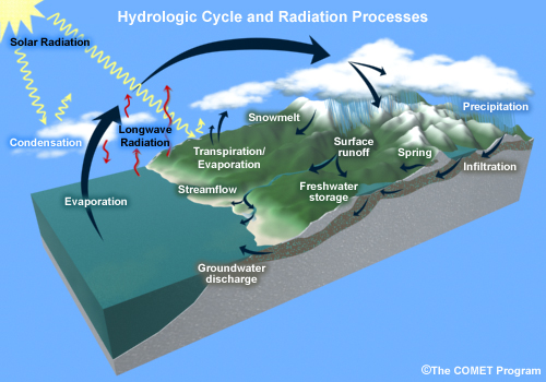
Water vapor constitutes 0-4% of the total volume of the atmosphere, yet it is the most important determinant of weather and climate. Figure 5.1 illustrates some processes that are critical to weather and climate in the tropics.
- First, water vapor condenses to form precipitation, an essential resource for life. The potential for precipitation is determined by the amount of water vapor. Keep in mind that entire economies in parts of the tropics depend on an adequate supply of fresh water.
- Second, water vapor is an active absorber and emitter of infrared radiation, thereby affecting heating and cooling of the atmosphere and surface.
- Third, latent heat release when vapor condenses or freezes is an important energy source for atmospheric motion and convective weather systems.
- Fourth, vertical transport of water vapor, through cumulus convection, is the most important mechanism for upward transport of heat in the tropics. Water vapor enters the atmosphere through surface evapotranspiration, whereby latent energy is absorbed. When the vapor condenses or freezes, the latent heat is released to the atmosphere.
- Fifth, the amount of water vapor influences the rate of surface evaporation and transpiration. Humans and other animals are uncomfortable in highly humid conditions that impede the rate of perspiration. Conversely, very low humidity leads to dehydration and related health problems.
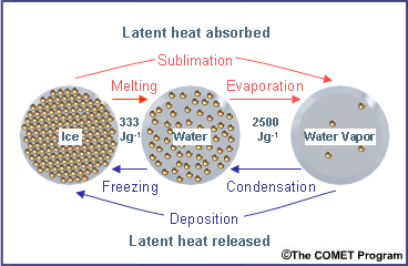
Furthermore, water is constantly changing phases (Fig. 5.2) within the range of normal atmospheric temperatures, which is unlike other atmospheric gases.
5.1 Atmospheric Moisture »
5.1.1 Importance of Water Vapor »
5.1.1.1 Measuring Water Vapor Content
Meteorologists describe the amount of water vapor in the atmosphere in terms of the vapor pressure, specific humidity, mixing ratio, relative humidity, and saturation (Box 5-1). Atmospheric moisture content is measured directly, using instruments such as hygrometers and psychrometers, or estimated from satellite microwave sensor measurements. Descriptions of the instruments and methods of observation for humidity and other weather elements are available from the World Meteorological Organization (WMO) Instruments and Methods of Observation Programme.
Meteorologists describe the amount of water vapor in the atmosphere in terms of the vapor pressure, specific humidity, mixing ratio, relative humidity, and saturation (Box 5-1). Atmospheric moisture content is measured directly, using instruments such as hygrometers and psychrometers, or estimated from satellite microwave sensor measurements. Descriptions of the instruments and methods of observation for humidity and other weather elements are available from the World Meteorological Organization (WMO) Instruments and Methods of Observation Programme.
5.1 Atmospheric Moisture »
5.1.1 Importance of Water Vapor »
Box 5-1 Defining Water Vapor Content
- Vapor pressure: The partial pressure of air that is exerted by water vapor (hPa or mb)
- Specific humidity: Mass of water vapor divided by the mass of air (g kg-1)
- Mixing ratio: Mass of water vapor divided by the mass of dry air (g kg-1)
- Dew point temperature: The temperature to which air must be cooled (at constant pressure and vapor content) for saturation to occur. The frost point temperature is similar except for saturation relative to ice (°C/°F/K)
- Relative humidity (RH): Ratio of specific humidity to saturation specific humidity. The amount of water vapor compared with the amount required for saturation (at a particular temperature and pressure).
- Saturation or equilibrium: Condition of the atmosphere when the evaporation rate is equal to the condensation rate. When air is saturated, the amount of water vapor is the maximum that can exist at a particular temperature and pressure.
For more information on moisture parameters see the COMET Skew-T Mastery module at http://www.meted.ucar.edu/mesoprim/skewt/
Observing Methods and, Automatic Weather Stations
http://www.wmo.int/pages/prog/www/IMOP/publications/CIMO-Guide/CIMO_Guide-7th_Edition-2008.html
5.1 Atmospheric Moisture »
5.1.2 Evaporation, Condensation, and Saturation
Let us imagine a parcel of air (one kg mass). Evaporation and condensation occur at the surface of small drops in the parcel. When the evaporation rate and condensation rate are equal, a state of saturation or equilibrium exists. If the air parcel is heated, the evaporation rate increases because the more energetic molecules can evaporate more easily. As the temperature increases, more molecules are needed to achieve equilibrium or saturation.
The function that describes the relationship between the saturation vapor pressure and temperature is the Clausius-Clapeyron equation:
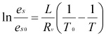 (1)
(1) where T is the temperature in K
To is 273K
es is the saturation water vapor pressure in hPa
eso is the saturation water vapor pressure at temperature To (6.11 hPa)
Lv is the latent heat of vaporization (2.453 × 10⁶ J kg-1), and
Rv is the water vapor gas constant (461 J kg-1 K-1).
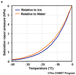
Note that values measured empirically, by in situ instruments, will differ from those calculated from the equation, as Lv is dependent on temperature. The Clausius-Clapeyron equation can be applied to any phase change. A similar equation can be obtained for saturation with respect to an ice surface by substituting Lv with the latent heat of sublimation (Fig. 5.2). The equation predicts a steeper curve for the vapor pressure over ice because the latent heat of sublimation is greater than the latent heat of vaporization at similar temperatures. These differences play a critical role in the formation of precipitation in clouds where water exists in ice and liquid phases.
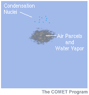
Saturation in the atmosphere is achieved through cooling to the dew point or frost point, adding moisture, or through the isobaric mixing of air with different temperature and moisture content (Fig. 5.3). Net condensation results in the formation of dew, haze, fog, or clouds. In the atmosphere, droplets form when vapor condenses on tiny particles which have an affinity for water; they are hygroscopic. The particles are called condensation nuclei (CN) and the process is called heterogeneous nucleation. Ice crystals form when the temperature is below the freezing point and ice is nucleated either by direct deposition from the vapor on nuclei, freezing on nuclei, contact freezing on nuclei (all heterogeneous nucleation), or by freezing of pure water vapor below -40°C (homogeneous nucleation). Super-saturation is the term used to describe the condition when relative humidity exceeds 100% and net condensation or deposition occurs.
5.1 Atmospheric Moisture »
5.1.3 Sources of Water Vapor: Evaporation and Evapotranspiration
Evaporation from the ocean is the primary means by which water and energy are transported from the surface to the atmosphere. The tropics drive the global energy and water cycle since the oceans, which comprise most of the tropical surface, receive a surplus of radiative heating. The significance of the tropical ocean as a source of water vapor is easy to imagine if you consider that the Pacific Ocean alone spans nearly one half of the earth's circumference at the equator. While evaporation over land is less than that over the ocean, its distribution plays a vital role in the initiation and evolution of convective weather systems. Tropical forested regions, like the Amazon, are significant sources of water vapor.
Following methods first introduced in the 1940s,1 evaporation over the ocean is estimated by an empirically-derived equation:
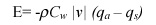 (2)
(2) where ρ is the air density
v is the wind velocity
qs is the saturation specific humidity at sea surface temperature
qa is the specific humidity at 10m above the surface
Cw is the coefficient of eddy diffusivity, a factor related to the roughness of the surface.
The coefficient Cw is altered to allow for very light winds (e.g., over the Tropical Pacific where the wind is near zero).
Evaporation can be measured using eddy correlation2 or eddy covariance techniques and relative humidity sensors that record changes on highly turbulent scales (sometimes less than 1 second). Evaporation rates are also estimated from satellite microwave sensors, which detect radiation emitted by water vapor, as described in Chapter 2. Standards for measurement of evaporation are provided by the WMO.
Evaporation can be measured using eddy correlation2 or eddy covariance techniques and relative humidity sensors that record changes on highly turbulent scales (sometimes less than 1 second). Evaporation rates are also estimated from satellite microwave sensors, which detect radiation emitted by water vapor, as described in Chapter 2. Standards for measurement of evaporation are provided by the WMO.
Where would you expect evaporation rates to be high? (Choose all that apply.)
The correct answers are b and c.
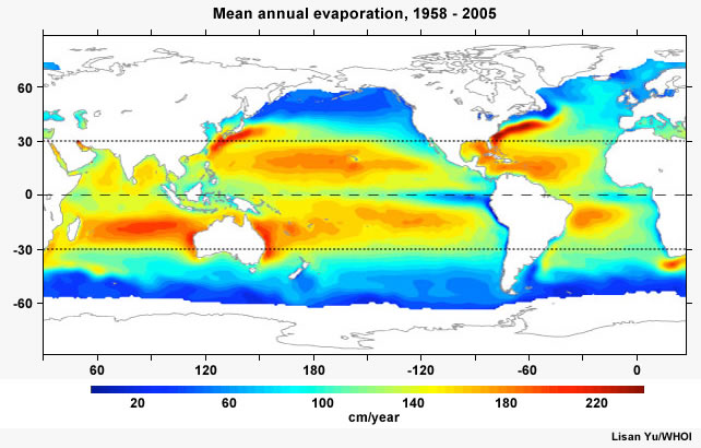
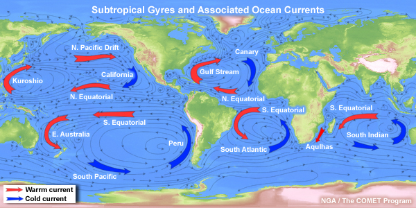
On average, regions equatorward of 30° latitude have much higher evaporation rates than higher latitude zones, a distinguishing feature of the tropics. The highest evaporation rate occurs along the western side of the subtropical oceans (Fig. 5.4) during the winter when cold, dry continental air flows over warmer ocean currents such as the Gulf Stream and Kuroshio. Stronger surface winds in winter also contribute to higher rates of evaporation. Evaporation rates increase in the inflow areas of hurricanes and where storms increase the wind speed over the ocean. Deep convective clouds increase the rate of evaporation because of the wind speed.
Why are evaporation rates so low along the equator, where solar heating is at the maximum?3 The lowest rates are found above cold currents and upwelling regions such as the equatorial eastern Pacific (Box 5-2). The latter is due to reversal of the sign of the Coriolis acceleration (Box 5-2). Another reason is that deep convective clouds reduce the amount of solar radiation.4 Wind speed and ocean transport are also partly to blame; low wind speeds in the equatorial oceans reduce the evaporation rates.5
Why are evaporation rates so low along the equator, where solar heating is at the maximum?3 The lowest rates are found above cold currents and upwelling regions such as the equatorial eastern Pacific (Box 5-2). The latter is due to reversal of the sign of the Coriolis acceleration (Box 5-2). Another reason is that deep convective clouds reduce the amount of solar radiation.4 Wind speed and ocean transport are also partly to blame; low wind speeds in the equatorial oceans reduce the evaporation rates.5
OAFlux Dataset, http://oaflux.whoi.edu/
Presentation on Evaporation Variability, Dr. Lisan Yu
5.1 Atmospheric Moisture »
5.1.3 Sources of Water Vapor: Evaporation and Evapotranspiration »
Box 5-2 Upwelling
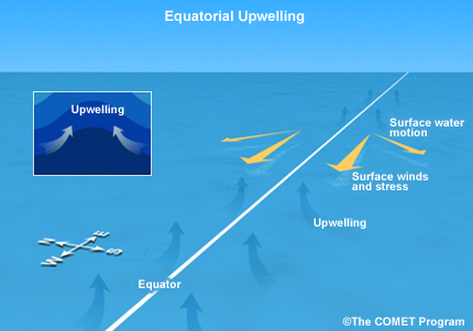
Upwelling brings cooler and denser water to the ocean surface. One of the primary places for upwelling in the tropics is along the equator (Fig. 5B2.1). Wind stress from the easterlies winds creates a current, which is deflected due to the Coriolis force: to the right (left) in the northern (southern) hemisphere. The resulting divergence of surface water brings cooler, deeper water to the surface and reduces the sea surface and air temperature.
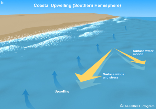
Upwelling also occurs along coasts where surface water is moved offshore in response to currents that flow along the coast, as illustrated for the southern hemisphere (Fig. 5B2.2). The northwest coast of South America is noted for strong upwelling.
An introduction to ocean currents and upwelling is provided in COMET module Introduction to Ocean Currents, http://meted.ucar.edu/oceans/currents/
5.1 Atmospheric Moisture »
5.1.3 Sources of Water vapor: Evaporation and Evapotranspiration »
5.1.3.1 Evapotranspiration
Another source of water vapor is transpiration, the process by which water vapor enters the atmosphere through the stomata in the leaves of plants. The contribution of water vapor from evaporation and transpiration combined is known as evapotranspiration (ET) and represents an important part of the water cycle (see Fig 5.1). ET rates for amply-watered plants are determined by:
- Incoming radiation: ET rates increase as incoming radiation increases
- Temperature: ET rates increase as temperature rises until an optimum temperature is reached. The optimal temperature varies by type of plant, with tropical plants typically having a higher optimum temperature than those at higher latitudes. As temperature increases above the optimum temperature, the ET rates decrease.
- Relative humidity: ET increases with the relative humidity gradient. The bigger the moisture gradient between the surface and the air, the higher the ET. As the relative humidity of the air rises, ET rates fall. Other things being equal, it is easier for water to evaporate into drier air than more moist air.
- Wind: Increased wind speed results in a higher ET rate in unstressed plants. With little movement of the air, water saturates air surrounding leaves or the air above water surfaces. With movement, saturated air is replaced by drier air. Note that evaporation happens even under calm conditions.
- Soil moisture availability: When soil moisture is lacking, plants transpire less, and can even wilt when the soil is very dry.
- Type of plant: Transpiration rates vary among plants. For example, plants in arid regions conserve water by transpiring less.
Potential evapotranspiration is a measure of the maximum possible water loss from an area under a specified set of weather conditions. Maximum annual potential evapotranspiration occurs where temperatures are highest in regions such as the Sahara Desert (Fig. 5.5). Values are very low where temperatures are low and vegetation is sparse, such as the Tibetan Plateau. Rates are relatively low where the surface-to-atmosphere moisture gradient is weak and relatively high where that gradient is strong. Evaporation pans and lysimeters are two common methods used to measure the potential evapotranspiration, which often greatly exceeds the actual ET.
WMO Web Portal on Development, Maintenance and Operation of Instruments,
Observing Methods and, Automatic Weather Stations
http://www.wmo.int/pages/prog/www/IMOP/publications/CIMO-Guide/CIMO_Guide-7th_Edition-2008.html
Evaporation measurement by evaporation pans and lysimeters,
http://www.meted.ucar.edu/hydro/basic/HydrologicCycle/print_version/03-atmospheric_water.htm#12
5.1 Atmospheric Moisture »
5.1.4 Distribution of Surface Water Vapor
Before proceeding, think about the following. Should the tropics have more or less water vapor than the mid-latitudes? Do you expect the values to be generally consistent around the globe? If not, what might cause variation?
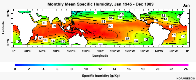
The Comprehensive Ocean-Atmosphere Data Set (COADS)6 maps show that specific humidity over the tropical oceans ranges from 3 to 24 g kg-1 (animation of Fig. 5.6). The highest values are found in June over the Arabian Sea and northern Indian Ocean. A broad band of high specific humidity is found near the equator and follows the seasonal cycle. However, specific humidity is not uniform along latitude zones. During January, the highest values occur over the equatorial west Pacific while the lowest values are found in the northwest regions of the Pacific and Atlantic. During July, the highest values occur over the northwest Pacific, Bay of Bengal, and the waters surrounding the Arabian Peninsula. Throughout the year, the eastern Pacific and eastern Atlantic have relatively low specific humidity poleward of 10° latitude. Relatively low values also occur along the equator over the central and eastern Pacific.
What causes these variations? (Type your response in the box below.)
Feedback:
Regions of low water vapor content are associated with the cold currents that flow from the poles along the west coasts of continents and upwelling of cold water at the equator.
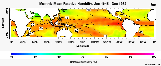
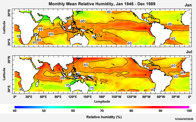
Relative humidity mimics the pattern of specific humidity for the equatorial trough region (Fig. 5.7). In this region, the abundance of surface moisture in combination with nearly constant high temperature leads to high specific humidity and high relative humidity. However, relative humidity can be high in regions where the specific humidity is low. For example, surface saturation specific humidity is low, but relative humidity is high, over the eastern, tropical ocean basins due to the cold ocean currents and upwelling.
Create COADS Data Plots, http://iridl.ldeo.columbia.edu/SOURCES/.COADS/
Create plots from Surface Marine Atlas, http://iridl.ldeo.columbia.edu/SOURCES/.DASILVA/.SMD94/
5.2 Adiabatic Processes and Vertical Distribution of Moisture
5.2 Adiabatic Processes and Vertical Distribution of Moisture »
5.2.1 Adiabatic Temperature Change
Imagine a parcel of air with a mass of 1 kg, which occupies a volume of about 1 m3, has an impermeable surface, and no heat exchange with the surrounding air. Where there is no energy gain or loss to the environment, any change in the volume of that parcel of air will result in a change in the internal energy of the parcel. This type of temperature change is said to be adiabatic.
Why is this process important in meteorology? As a rising air parcel encounters lower pressure, its volume increases and its internal energy decreases because energy is needed to expand against the surrounding air. A reduction in the internal energy per unit volume causes the temperature to fall at what is known as the dry adiabatic lapse rate (0.98°C per 100 m ≈ 10°C per km). If the temperature continues to decrease until the parcel reaches its dewpoint temperature, condensation occurs. Further cooling occurs at the saturated adiabatic lapse rate, which is a slower rate of cooling because of the latent heat release that occurs with condensation.
When an air parcel sinks, it is compressed by the surrounding air. As the volume decreases, the internal energy increases, the temperature increases, and the relative humidity decreases.
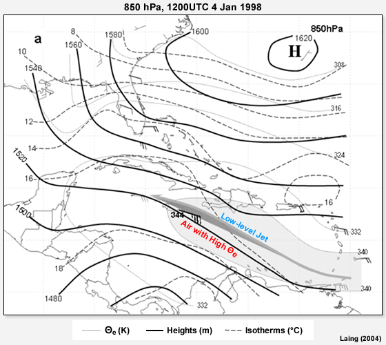
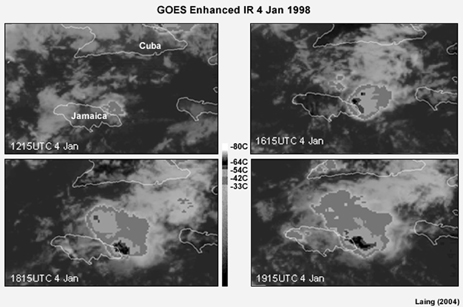
Sometimes it is convenient to use the potential temperature, θ instead of the temperature because every parcel of air has a unique value of potential temperature that remains the same while the parcel is rising or sinking dry adiabatically. With a saturated air parcel, we assume that all condensate will eventually fall out. This process is referred to as pseudo-adiabatic (some latent heat is removed with the precipitation) and the equivalent potential temperature, θe, remains the same. In order to predict heavy precipitation from convection, forecasters look at the movement of the air with high values of θe. For example, in Fig. 5.8, heavy rainfall occurred within the axis of maximum θe at 850 hPa.7 In this case, the maximum rainfall and deadly flash floods were produced where the high θe air was lifted along the mountains in eastern Jamaica.
You can review potential temperature, θ, and equivalent potential temperature, θe, and other thermodynamic variables in the COMET module Skew-T Mastery at http://meted.ucar.edu/mesoprim/skewt.
5.2 Adiabatic Processes and Vertical Distribution of Moisture »
5.2.2 Tropical Clouds
5.2 Adiabatic Processes and Vertical Distribution of Moisture »
5.2.2 Tropical Clouds »
5.2.2.1 Tropical Cloud Formation and Types
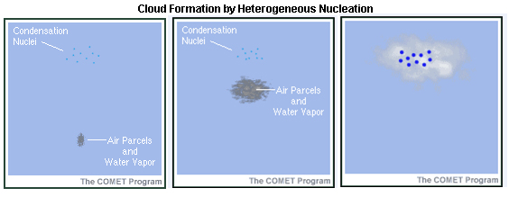
Clouds form when air is lifted to its saturation point by fronts, topography, convergence, or convection. As mentioned in Section 5.1.2, cloud droplets form with the aid of cloud condensation nuclei or CCN (Fig. 5.9). Some CCN are more hygroscopic than others-allowing condensation at relative humidity values below 100%. Warm clouds have temperatures greater than 0°C, while cold clouds are colder than 0°C. Mixed-phase clouds have ice crystals and super-cooled droplets. Below -40°C, clouds consist entirely of ice.
Clouds form when air is lifted to its saturation point by fronts, topography, convergence, or convection. As mentioned in Section 5.1.2, cloud droplets form with the aid of cloud condensation nuclei or CCN (Fig. 5.9). Some CCN are more hygroscopic than others-allowing condensation at relative humidity values below 100%. Warm clouds have temperatures greater than 0°C, while cold clouds are colder than 0°C. Mixed-phase clouds have ice crystals and super-cooled droplets. Below -40°C, clouds consist entirely of ice.
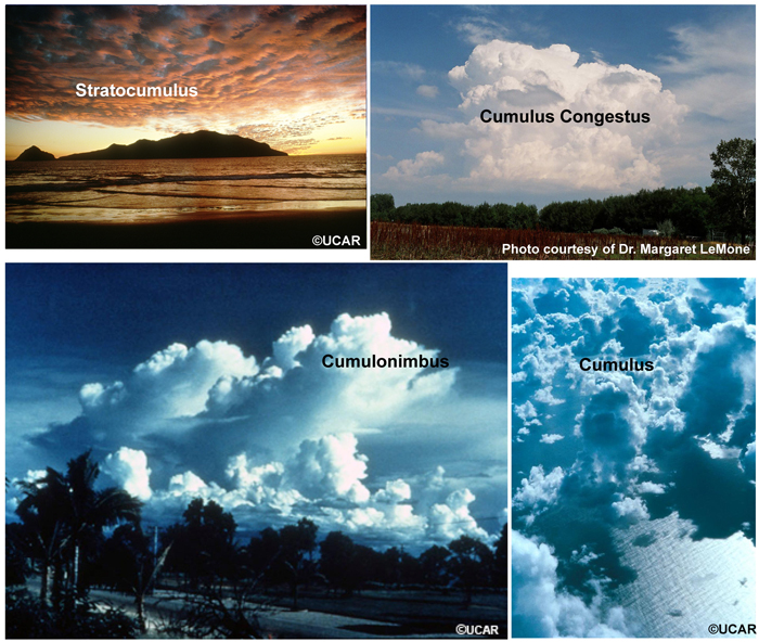
The tropical cloud layer is dominated by cumuliform clouds: shallow cumulus, stratocumulus, cumulonimbus, and cumulus congestus (e.g., Fig. 5.10, below).
5.2 Adiabatic Processes and Vertical Distribution of Moisture »
5.2.2 Tropical Clouds »
5.2.2.2 Cumulus convection
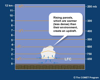
Convection associated with cumulus clouds (or cumulus convection) refers to the process by which an air parcel is heated, expands, becomes less dense than the surrounding air, is pushed upward to its saturation point, and forms a cloud or convective cell. The upward acceleration of air parcels creates an updraft. The force that causes parcels to accelerate upward is called buoyancy and it is proportional to the density difference between the rising parcels and their environment.
Convection associated with cumulus clouds (or cumulus convection) refers to the process by which an air parcel is heated, expands, becomes less dense than the surrounding air, is pushed upward to its saturation point, and forms a cloud or convective cell. The upward acceleration of air parcels creates an updraft. The force that causes parcels to accelerate upward is called buoyancy and it is proportional to the density difference between the rising parcels and their environment.
The height at which a lifted parcel first becomes warmer (less dense) than the surrounding air is referred to as the Level of Free Convection (LFC). Once the parcel reaches the LFC, it continues to rise freely until it becomes as cool (as dense) as the surrounding air. This upper level is the Equilibrium Level (EL).
The vertically integrated buoyancy between the LFC and the EL is referred to as the Convective Available Potential Energy or CAPE.8,9 The CAPE is the positive area between the ambient temperature profile and the moist adiabat connecting the LFC and the EL on a Skew-T-log P diagram (Fig. 5.11).
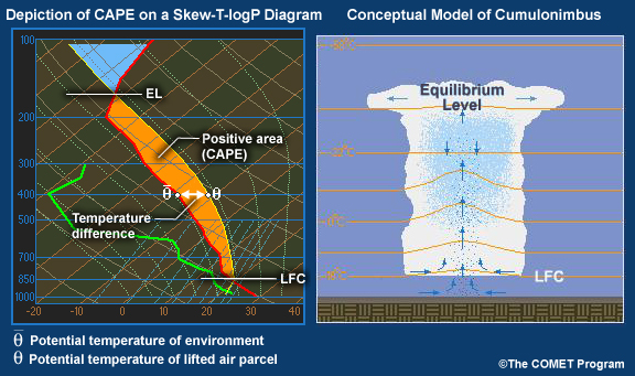
The CAPE, measured in joules per kilogram (J kg-1), can be calculated using Equation 3,
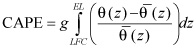 (3)
(3)where g is the acceleration due to gravity (m s-1), z is altitude (m), θ is the potential temperature of the lifted air parcel (K), and θ is the potential temperature of the environment (K).
The CAPE for thunderstorms is often in the range of 1000-2000 J kg-1 although it can exceed 4000 J kg-1 in severe thunderstorms and be as small as 700 J kg-1 in shallow trade cumuli. CAPE is a useful parameter for diagnosis of convection because it is directly related to the maximum potential speed, Wmax, of the updraft.
 (4)
(4)Updraft velocities over tropical oceans, where the parcel-environment temperature difference is 1K or less10,11 are slower than in severe thunderstorms over the mid-latitude continents where the temperature difference is several degrees. In reality, Wmax can be reduced by as much as a factor of 2 because the measure of buoyancy using only temperature difference does not account all effects. CAPE is not always an accurate estimator of the contribution to buoyancy in deep convective storms12,13 because of effects such as variations in the liquid water load and entrainment, which is the integration of environmental air into the turbulent cloud-scale circulation.
On reaching the equilibrium level, parcels do not stop abruptly. Rather, they oscillate about their equilibrium level and then spread out to form an anvil-shaped cloud top.
During ascent through the cloud, parcels gain water droplets or ice (depending on the temperature). Eventually the water droplets or ice crystals become heavy enough to fall or precipitate out of the cloud. Falling precipitation and the cool air it drags down form a downdraft. The cooler the downdraft, the faster it accelerates downward. Evaporation of rain beneath the cloud base cools the downdraft further, forming a "cold pool" that spreads out rapidly from the convective cell. The cold pool (also referred to as an outflow boundary or gust front) in the tropics is much weaker than in the midlatitudes except in large tropical squall lines.
The final stage of the convective cell is dominated by downdrafts and negative buoyancy. New cells form as air is lifted over the boundary of the cold pool. The stages of moist continental convection are illustrated in Fig. 5.12.
Learn more about buoyancy and CAPE in the module Principles of Convection: Buoyancy and CAPE, http://www.meted.ucar.edu/mesoprim/cape/index.htm. Tropical convection will be explored further in subsequent chapters.
5.2 Adiabatic Processes and Vertical Distribution of Moisture »
5.2.2 Tropical Clouds »
Box 5-3 Buoyancy
Consider a rising parcel (Fig. 5B3.1) of with temperature, Tparcel, volume, Vparcel, and density, ρparcel, that displaces an equal volume of ambient air with temperature, Tenv, and density, ρenv. The net buoyant force or buoyancy, a function of the difference in density between the air parcels, is expressed as a force per unit mass,
 (B5-3.1)
Note that this measurement is an overestimate as it neglects the effects of decreasing water vapor and increasing condensed water, which reduce the buoyancy, especially in the tropics.
5.2 Adiabatic Processes and Vertical Distribution of Moisture »
5.2.2 Tropical Clouds »
5.2.2.3 Tropical Cloud Population and Distribution
The amount of clouds in a particular region depends on the relative humidity and the availability of mechanisms for lifting air to saturation. Therefore, the Inter-tropical Convergence Zone (ITCZ)14 and the Asian MonsoonAsian Monsoon regions have large cloud amounts while the subtropical highs have relatively low cloud amounts, with the lowest in the Sahara Desert (Fig. 5.13). Yet some areas within the subtropical high pressure belt have very high cloud amounts. For example, cloud amounts in subtropical eastern Pacific and eastern Atlantic exceed 70%.
What could be contributing to the large amount of cloudiness in these areas? Do you think that the clouds in the eastern Pacific and eastern Atlantic are the same types of clouds as those in the ITCZ? (Type your response in the box below.)
Feedback:
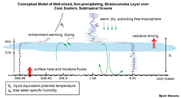
Recall the distribution of surface relative humidity (Fig. 5.7). The eastern boundaries of the tropical oceans are marked by cold currents and upwelling as surface water is transported westward in response to the easterly trade winds. Stratocumulus clouds form within the resulting cool, moist boundary layer. Predominantly high pressure, sinking air, and adiabatic warming cause temperature to increase with height above the relatively-shallow, cool boundary layer. Profiles of the liquid equivalent potential temperature, θl, and the total water specific humidity, qt, illustrate the dramatic difference between the cool, moist boundary layer and the warm, dry free atmosphere (Fig. 5.14).15
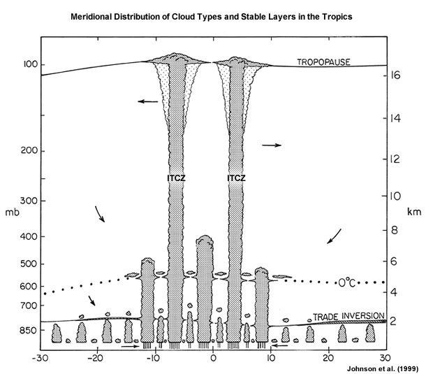
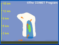
Observations from the Tropical Ocean Global Atmosphere Coupled Ocean-Atmosphere Response Experiment (TOGA COARE)16 illustrate the change in cloud type and depth as one approaches the equator from the subtropics. Cloud depth varies with the depth of the trade wind inversion Cloud depth varies with the depth of the trade wind inversion.14,17 Cloud types vary from shallow cumulus to cumulus congestus and cumulonimbus in the ITCZ18 (Fig. 5.15). Similar trends in cloud population and depth exist across the central and east Pacific, except that there is a single ITCZ (Fig. 5.16).
Shallow cumuli often congregate into lines, clusters19,20 or cells21 while cumulonimbus are often organized into mesoscale (+100 km scale) systems22,23,24 such as those seen within the ITCZ in Fig. 5.16.
http://loaamma.univ-lille1.fr/AMMA/
Lecture: Clouds in the equatorial trough zone, Prof. Robert Houze
http://www.asp.ucar.edu/colloquium/2001/houze.pdf
http://cimss.ssec.wisc.edu/wxwise/gifs/LWALL.mpg
and monthly mean albedo,
http://cimss.ssec.wisc.edu/wxwise/gifs/ALBALL.mpg
5.2 Adiabatic Processes and Vertical Distribution of Moisture »
5.2.3 Thermodynamic or Static Energy
The movement of energy from the tropical surface to the atmosphere is an important part of the global energy cycle. In this section, we will examine the energy within an air parcel. Specifically, we will consider what is referred to as the thermodynamic or static energy, which is a sum of the following:
- Potential energy, which is associated with the gravitational force or position relative to the center of the earth
- Sensible heat or internal energy, which depends on temperature
- Latent heat, which is absorbed or released during the phase change of water
Thermodynamic energy is conserved by individual air parcels during adiabatic vertical motion and can be described in equation form as:
Dry static energy = sensible heat + geopotential
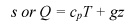 (5)
(5)Moist static energy = sensible heat + geopotential + latent heat
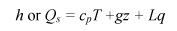 (6)
(6)where L is latent heat; cp is specific heat at constant pressure; g is acceleration due to gravity; and z is altitude.
The moist static energy and the equivalent potential temperature, θe, are sometimes used interchangeably because of this relationship:25
 (7)
(7)Here, T is the temperature of the condensation level. It is assumed that all condensate falls out immediately. This approximation is least accurate in the upper troposphere of the tropics.25
The moist thermodynamic or static energy of the tropical atmosphere, which is illustrated using profiles of θe, has a minimum in the middle troposphere26 (Fig. 5.17).
Which profile represents an environment in which large thunderstorm systems with heavy precipitation are prevalent? (Choose the best answer.)
The correct answer is d.
As the amount of precipitation increases, the moist static energy in the low to middle troposphere increases. Between 700 and 600 hPa, θe increases from 316K to 335K as conditions vary from fair weather to widespread heavy rain. Near surface θe also increases but only by a few degrees.
As the average value of θe changes, so do the profiles. How do the profiles vary? (Type your response in the box below.)
Feedback:
The moist static energy minimum occurs at a higher altitude and the vertical gradient is much less for profiles inside the convection than in environmental profiles.
Figure 5.18 illustrates the dramatic difference between the thermodynamic energy of fair weather environments and environments with widespread deep convection and rain. The temperature varies little, therefore much of the difference is due to the moisture content in the lower and mid-troposphere. Similar changes are observed ahead and in the wake of large convective systems.
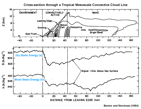
While mid-troposphere moist static energy is the most prominent indicator of rainfall amount significant changes can occur at the surface. Both the moist static energy, h, and dry static energy, s, decrease abruptly during the passage of the leading edge of a strong mesoscale convective cloud line (Fig. 5.19). While s starts to increase after its passage, h continues to decrease even though the rainfall decreases in intensity. In the wake of the most intense precipitation, both s and h gradually increase to their starting value more than 160 km behind the leading edge.
5.2 Adiabatic Processes and Vertical Distribution of Moisture »
5.2.4 Mean Thermodynamic Profiles of the Tropical Atmosphere
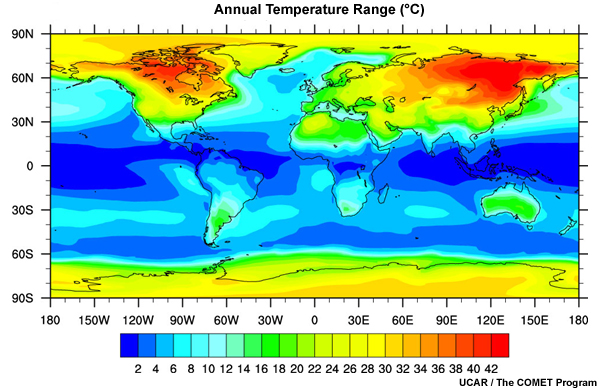
Compared with the midlatitudes, the tropical atmosphere is fairly steady. For example, the annual range of land surface temperature is less than or equal to the average daily range. Thus, it is tempting to think that mean thermodynamic conditions over the tropical oceans could be represented by a single sounding. In fact, mean thermodynamic conditions are varied. Profiles of relative humidity (Fig. 5.20), potential temperature and equivalent potential temperature (Fig. 5.21) illustrate variations over the Caribbean,29,30,31 tropical north Atlantic and tropical west Pacific32,33 and eastern Arabian Sea.34
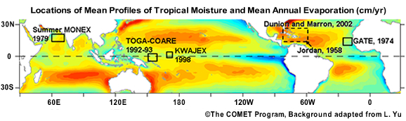
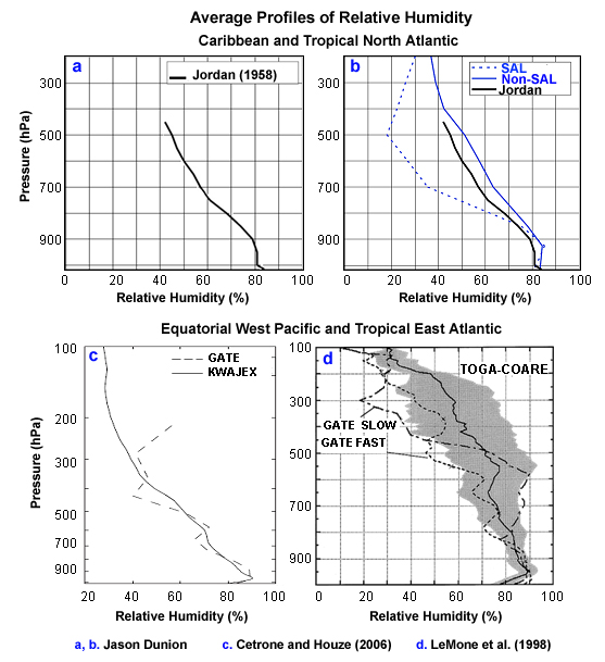
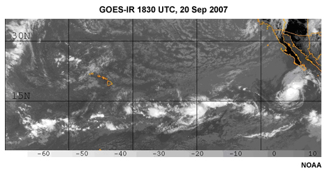
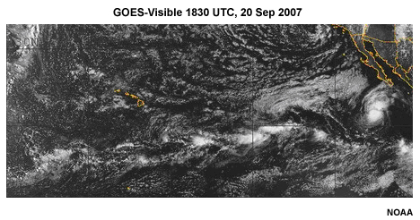
The mean sounding calculated by Jordan in 1958 (Fig. 5.20a, Fig. 5.21a) has often been used as a standard profile for the tropics. That mean sounding was calculated from soundings over the Caribbean. Updated mean soundings have been calculated from a larger set (770) of soundings by Dunion and Marron31 (Fig. 5.20b, Fig. 5.21b). In comparison to the updated mean sounding data by Dunion and Marron, the Jordan mean sounding is too dry in the low-mid troposphere (Fig. 5.20b). One of the contributors to to dry air in the low-middle troposphere is the Saharan Air Layer (SAL). The influence of the SAL was observed during the Global Atmospheric Research Program (GARP) Atlantic Tropical Experiment (GATE), held in the tropical eastern Atlantic and West Africa in 1974. The SAL is a dry and often very dusty air mass that forms when air is lifted from the desert during dust storms.31 Although dust storms can occur at any time, they are more common between late spring and early autumn. The driest layer occurs between 1500-6000 m and moves across the Atlantic above moist, relatively cool, low-level air. The effect of the SAL is seen in the mean GATE sounding where the low-to-mid troposphere is much drier than over the tropical, west Pacific (Fig. 5.20c). Chapter 2, Section 2.8, describes how the SAL and other dust layers are tracked using satellite remote sensing.
The mean sounding calculated by Jordan in 1958 (Fig. 5.20a, Fig. 5.21a) has often been used as a standard profile for the tropics. That mean sounding was calculated from soundings over the Caribbean. Updated mean soundings have been calculated from a larger set (770) of soundings by Dunion and Marron31 (Fig. 5.20b, Fig. 5.21b). In comparison to the updated mean sounding data by Dunion and Marron, the Jordan mean sounding is too dry in the low-mid troposphere (Fig. 5.20b). One of the contributors to to dry air in the low-middle troposphere is the Saharan Air Layer (SAL). The influence of the SAL was observed during the Global Atmospheric Research Program (GARP) Atlantic Tropical Experiment (GATE), held in the tropical eastern Atlantic and West Africa in 1974. The SAL is a dry and often very dusty air mass that forms when air is lifted from the desert during dust storms.31 Although dust storms can occur at any time, they are more common between late spring and early autumn. The driest layer occurs between 1500-6000 m and moves across the Atlantic above moist, relatively cool, low-level air. The effect of the SAL is seen in the mean GATE sounding where the low-to-mid troposphere is much drier than over the tropical, west Pacific (Fig. 5.20c). Chapter 2, Section 2.8, describes how the SAL and other dust layers are tracked using satellite remote sensing.
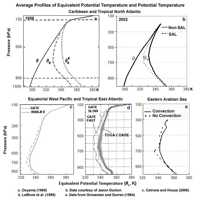
Soundings from GATE, TOGA-COARE, and KWAJEX, show that greater moist thermodynamic or static energy exists over the tropical west Pacific than over the tropical east Atlantic (Figs. 5.21c,d). The difference is due mainly to the higher average SSTs in the Pacific (29.1°C compared to 27-28°C in the east Atlantic).32 Convective systems in the two regions sometimes duplicate the moisture characteristics of the overall average soundings. For example, Fig. 5.20d shows that GATE fast moving convective lines were drier than west Pacific convective lines, similar to the overall mean profile (Fig. 5.20c). However, slow-moving GATE convective lines had relative humidities greater than 80% up to 600 hPa.
Differences in the vertical distribution of moisture within regions are dictated by the presence or absence of precipitating convection and what part of the convection is profiled. Note the difference between convective and non-convective environments over the eastern Arabian Sea (Fig. 5.21e). The vertical distribution of moisture is also affected by dry intrusions from midlatitude cyclones, which occasionally extend into the tropics.35,36 More information on the thermodynamic energy observed in various tropical field projects can be found in Lucas and Zipser (2000).27
![]()
CIMSS Real-time analyses of the SAL,
http://tropic.ssec.wisc.edu/real-time/salmain.php?&prod=splitEW&time
5.3 Precipitation
5.3 Precipitation »
5.3.1 Precipitation Processes
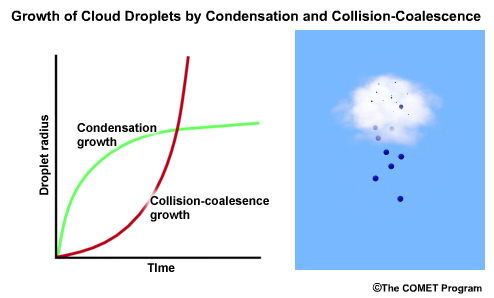
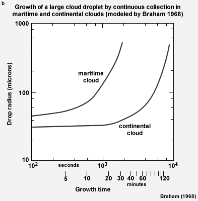
Most tropical precipitation falls as rain—as expected since most of the surface and lower troposphere are above freezing. A typical raindrop has a radius of about 1 mm while typical cloud droplet radii are 10s of µm.37 How do cloud droplets become raindrops? Cloud droplets do not grow large enough by condensation because the rate of growth of increase in droplet radius slows with time37 (Fig. 5.22). Warm cloud droplets grow and form precipitation by the collision-coalescence process38 (Fig. 5.22). Large droplets settle through small droplets and grow as small droplets collide and adhere to them.
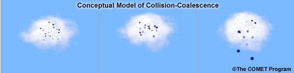
Collision-coalescence is most efficient in clouds that have a large distribution of condensation nuclei sizes and a deep, saturated warm layer. These conditions occur frequently in moist tropical areas, resulting in abundant rainfall. However, many tropical clouds that are capped by low level inversion (Fig. 5.15),18 such as trade wind cumuli, can exist without precipitating (or with low efficiency precipitation). For example, during the Rain in Cumulus over the Ocean (RICO)16 field program, clusters of trade cumuli would undergo growth, decay, and new cell formation without precipitating for hours. At various times during the cloud system lifetime, a "turret" would pop up out of the cluster and within 10s of minutes, precipitation would occur. The onset and evolution of precipitation in shallow tropical clouds is actively being studied in order to understand the relative influence of microphysics and turbulence, which influences vertical motion.15
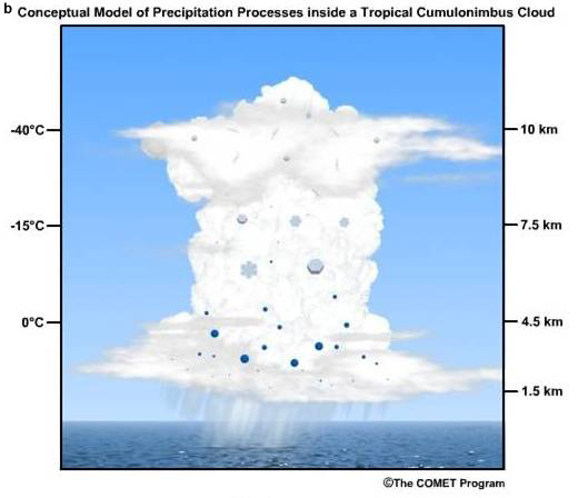
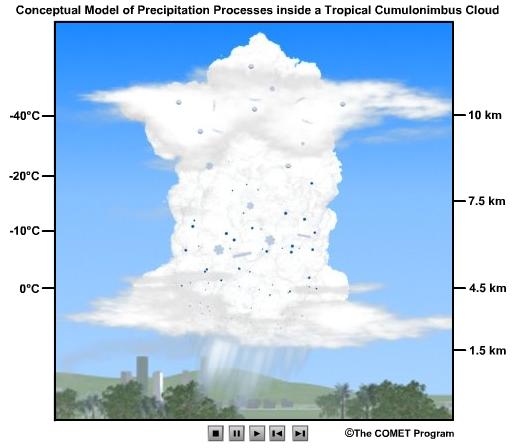
In cold clouds, ice crystals grow by deposition, riming, and aggregation. In mixed-phase clouds, ice grows rapidly at the expense of the liquid because the saturation vapor pressure is lower with respect to ice than water (Fig. 5.23a)—a process known as the Bergeron-Findeisen process. In cumulonimbus, which are common across equatorial continental regions and oceanic ITCZs,39 warm and cold processes contribute to precipitation (Fig. 5.23b).
Animation showing precipitation process over ocean.
Animation showing precipitation process over continents.
http://profhorn.meteor.wisc.edu/wxwise/precip/precip.html
Rain in Cumulus over the Ocean (RICO), http://www.eol.ucar.edu/projects/rico/
5.3 Precipitation »
5.3.2 The Impact of Aerosols: Maritime and Continental
The microphysical processes that lead to precipitation are affected by the aerosol present; in particular, the number of CCN has a large impact. In general, continental air has higher concentrations of CCN than maritime air and therefore continental clouds have higher droplet concentrations compared to maritime clouds.40 For a given amount of liquid water, many aerosol particles lead to many small droplets while fewer aerosols lead to a few large droplets (Fig. 5.24a). A reduction in droplet size range leads to fewer collisions. Therefore, droplets in maritime clouds are more likely to grow by collision and coalescence than droplets in continental clouds41 (Fig. 5.24b).
Aerosol effects on clouds and precipitation are complex and are actively being studied. For example, changes in the number and sizes of CCN can enhance or inhibit precipitation depending on the circumstances. Precipitation can be inhibited where continental aerosols are copious, such as downwind of cities, oil fires, or biomass burning42,43,44 while the addition of a few large CCN can enhance precipitation.45
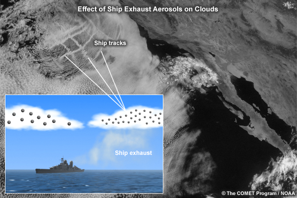
Furthermore, the surface area of many small droplets leads to more light scattering and makes the clouds with continental aerosols brighter.46,47 This phenomenon is clearly demonstrated by clouds that form downstream of ship exhausts. These clouds are commonly identified as "ship tracks" in satellite images (Fig. 5.25).
The relative amounts of solar radiation that a cloud reflects or absorbs is an indication of the size of its aerosols. The total amount of reflected light divided by the total amount of absorbed light is inversely proportional to the "effective radius" (reff ) of the cloud.48 For a given liquid water content, larger droplets reflect less but absorb more than smaller droplets. In warm clouds, reff is the sum of the volume of all drops divided by the sum of their surface area. Cloud droplets with reff greater than 14 µm are usually precipitating.38 Using reff and its relationship to satellite-retrieved cloud top temperature (T), it is possible to define five microphysical zones in deep convective clouds,48 although a given cloud will not necessarily conform to this idealized model (Fig. 5.26):
- Diffusional droplet growth zone, where droplets grow by condensation
- Region of droplet growth by coalescence
- Rainout region, where the effective radius is stable. Growth by coalescence is balanced by loss of the larger droplets; the cloud is raining while growing
- A mixed-phase region
- A glaciated zone
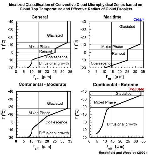
In reference to the conceptual relationships in Fig. 5.26, nearly all cloud droplets are nucleated at the base of convective clouds and then grow mostly by diffusion.48,49 Continental clouds have a smaller reff at cloud base, a well-developed diffusional growth zone, and colder mixed phase zone than maritime clouds (Fig. 5.26c). The depth of the diffusional zone is a measure of the "continentality" of a cloud. In the extreme (polluted) continental case (Fig. 5.26d), the coalescence zone disappears and the mixed phase zone is very cold. For maritime clouds, reff is large at cloud base, the diffusional zone is negligible, and the rainout zone is deep (Fig. 5.26b). Droplets grow faster above cloud base, implying that coalescence is a more dominant process in maritime clouds than in continental clouds. Maritime clouds glaciate at about -10°C while continental clouds typically glaciate below -15°C. Smoke-filled clouds glaciate at -20°C to -25°C.49
In addition to the size of aerosol, the mineral content can also affect the condensation rate, subsequent precipitation and cloud lifetime. For example, chemical transformations between fresh and aged smoke can change CCN activity and cloud characteristics.50 In 2005, scientists studied these effects by comparing areas of the tropical Atlantic that had mostly marine aerosols (30°-20°S), smoke (20°S-5°N), and mineral dust (5°-20°N). With the use of satellite images they found that smoke and mineral dust tend to suppress precipitation but increase the cloud coverage.51
The complex nature of aerosol effects is further illustrated by the finding that soot aerosols can increase dark haze and reduce the amount of trade cumulus over tropical oceans.52 Another study found that sea spray can restore precipitation in polluted convective clouds if winds and vertical motion are favorable.53 Finally, it should be noted that precipitation processes are influenced not only by aerosol effects but by dynamical processes such as turbulent mixing of cloud particles.
5.3 Precipitation »
5.3.3 Classification of Tropical Precipitation
Having examined the general processes of precipitation formation, it is natural to consider other properties of precipitation, such as precipitation rate, amount, duration, spatial distribution, temporal distribution, and the organization of precipitation systems.
Which of the following do you think accurately describes tropical rainfall? (Choose the best answer.)
The correct answer is d.
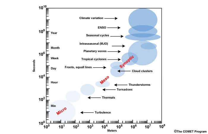
Most of the precipitation in the tropics is produced by organized cloud systems of length scale 100-1000 km whose lifetime ranges from several hours to a day.18,24 A thunderstorm system of this scale is called a mesoscale convective system (MCS).18,20,22
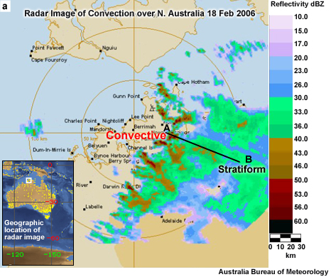
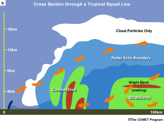
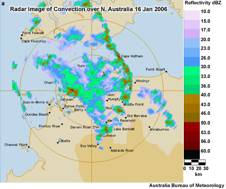
Precipitation from MCSs is usually classified as convective and stratiform.54 The convective classification refers to regions where precipitation is falling from active convection.24 Cloud particles grow by coalescence and/or riming in these regions of strong updrafts. Stratiform precipitation refers to older, less active convection. Vertical motion is generally weaker and particles grow mainly through deposition.55 The fraction of stratiform precipitation in MCSs increases with time during their lifecycle. The squall line with trailing stratiform precipitation is the most frequently studied type of MCS. Figure 5.27a shows a radar image of a tropical squall line with convective precipitation cells and a trailing region of stratiform precipitation. Figure 5.27b is a conceptual model of the vertical cross-section and profile of radar reflectivity through the squall line. Box 5-4 presents the typical lifecycle of a tropical squall line.
Precipitation from MCSs is usually classified as convective and stratiform.54 The convective classification refers to regions where precipitation is falling from active convection.24 Cloud particles grow by coalescence and/or riming in these regions of strong updrafts. Stratiform precipitation refers to older, less active convection. Vertical motion is generally weaker and particles grow mainly through deposition.55 The fraction of stratiform precipitation in MCSs increases with time during their lifecycle. The squall line with trailing stratiform precipitation is the most frequently studied type of MCS. Figure 5.27a shows a radar image of a tropical squall line with convective precipitation cells and a trailing region of stratiform precipitation. Figure 5.27b is a conceptual model of the vertical cross-section and profile of radar reflectivity through the squall line. Box 5-4 presents the typical lifecycle of a tropical squall line.
How do tropical rainfall rates differ from midlatitude rainfall rates? (Type your response in the box below.)
Feedback:
In general, tropical rainfall rates are much greater than midlatitude rainfall rates. However, the convective rain rates in severe thunderstorms and flash-flood producing MCSs are similar in both latitudinal zones.
Convective and stratiform precipitation rates in MCSs across the global tropics are derived from measurements by the Tropical Rainfall Measurement Mission (TRMM)57 Precipitation Radar (PR), the first satellite-precipitation radar. On average across the tropics, the ratio of convective to stratiform rain rate is 4 to 1 (Table 2).58 Over land, convective rain rates are an order of magnitude greater than stratiform rain rates. Although stratiform rain accounts for only 40% of the total rain, areas with stratiform precipitation rates cover about twice as much area as those with convective precipitation rates (Table 1).
| Stratiform rain fraction (%) | Stratiform area fraction (%) | Convective rain rate (mm h-1) | Stratiform rain rate (mm h-1) | Ratio of convective-stratiform rain-rate | |
| All | 40 | 73 | 7.3 | 1.8 | 4.1 |
| Land | 35 | 75 | 10.2 | 1.8 | 5.5 |
| Ocean | 43 | 72 | 5.8 | 1.8 | 3.3 |
(Adapted from Schumacher and Houze58)
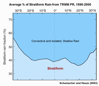
The percentage of stratiform rain increases with latitude beyond 20° of the equator but exceeds the convective rain amounts only south of 30°S (Fig. 5.28). Within 20° of the equator, less than 40% of the accumulated precipitation is stratiform; convective precipitation produces most of the rainfall in the equatorial zone.
A third category of tropical precipitation is shallow convective precipitation produced by cloud systems that are not organized as MCSs.
5.3 Precipitation »
5.3.3 Classification of Tropical Precipitation »
Box 5-4 Lifecycle of a Tropical Squall Line with Trailing Stratiform Region

The animation above is a conceptual model of tropical squall line cross-sections as the squall line moves from east to west (Fig. 5B4.1). The white areas represent the outline of the clouds and the blue represents the precipitation areas. The arrows indicate air flow with respect to the storm motion. The heaviest precipitation is found in the tall convective cells near the front of the system, whose highest reflectivity is represented by red-colored towers.
From an initial convective cell, the system grows, intensifies, and its structure becomes more complex. As the system matures, new convective cells develop along the outflow boundary (or gust front) of the old cells, and the old cells decay. A broad region of stratiform precipitation develops to the rear of the system-denoted by the broad green region. The line of bright red within the stratiform precipitation region indicates high reflectivity associated with the melting of ice crystals into raindrops.54 Unlike an ordinary, single cell thunderstorm (Fig. 5.12), this multi-cellular system is able to last for several hours because of new cell formation and the separation of its updraft from the downdrafts. The system is sustained by a warm, moist front-to-rear updraft from the leading edge. Downdrafts are created by precipitation and a rear-to-front flow in the mid-troposphere. This structure is common in squall lines all over the tropics. Although not shown here, vertical wind shear also exerts great influence on MCS organization.20
Below is an MCS, observed during the 2006 African Monsoon Multidisciplinary Analysis (AMMA)56 field program, that exhibited similar structure as it propagated west-southwestward (Figs. 5B4.2, 5B4.3).
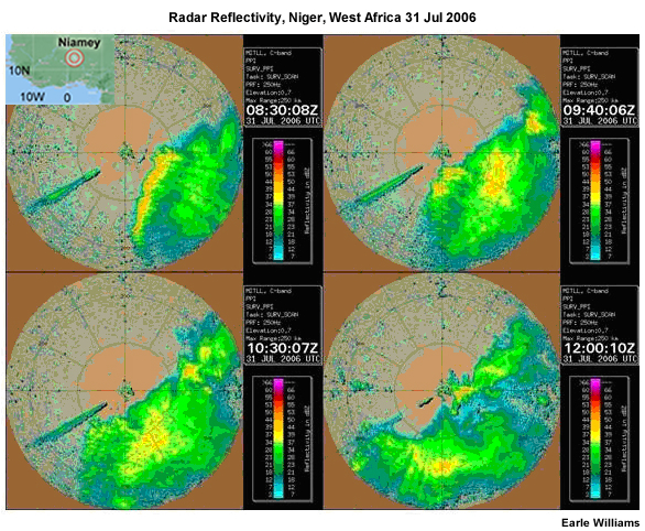
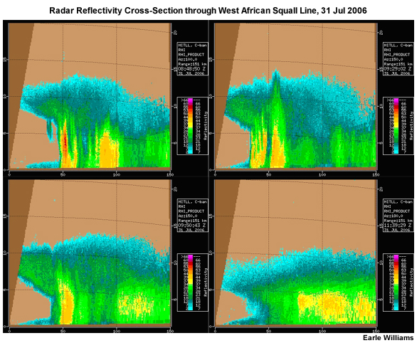
Radar images are from the Massachusetts Institute of Technology (MIT) radar, which operated in Niamey, Niger in support of the AMMA program. Images are courtesy of Dr. Earle Williams.
While the prevailing motion in the tropics is east to west, MCSs also move from west to east under the influence of varying vertical wind shear.20,32 Figure 2.8 of Chapter 2 displays tropical MCSs under easterly and westerly wind regimes.
5.3 Precipitation »
5.3.3 Classification of Tropical Precipitation »
Box 5-5 Measurement of Tropical Precipitation
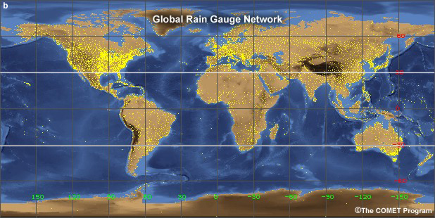
Precipitation over an area is usually estimated from a network of rain gauges (Fig. 5B5.1). Most gauges are placed near permanent settlements rather than distributed evenly. Thus, gauge-only maps are missing data over the ocean or inaccessible locations. Types and location of gauges produce additional sources of uncertainties.59 Since precipitation is unevenly distributed in space and time, its analysis presents challenges.
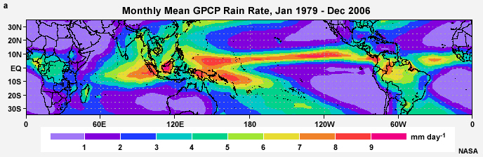
The Global Precipitation Climatology Project (GPCP)60 was established by the World Climate Research Program (WCRP) in 1986 to create community analysis of global precipitation. The GPCP is a merged analysis that incorporates precipitation estimates from low-orbit satellite microwave data, geosynchronous-orbit satellite IR data, and surface rain-gauge observations.61 Other popular datasets are CMAP62 and CMORPH.63
The Tropical Rainfall Measurement Mission (TRMM)57 Precipitation Radar, the first satellite-precipitation radar, has produced a rich dataset of precipitation rates58 and the vertical structure of precipitation in previously data-void regions.39,64 The TRMM Microwave Imager improves on microwave sensing technology pioneered by the Defense Meteorological Satellite Program Special Sensing Microwave Imager (SSM/I) in 1987 (Chapter 2, Section 2.5.3).
The future Global Precipitation Mission (GPM) is a satellite mission aimed at improving the spatial and temporal sampling of precipitation. GPM plans a constellation of satellites that will provide three-hourly views of about 80% of the globe (Chapter 2, Focus Section 2).
GPCP, http://www.gewex.org/gpcp.html
Global Precipitation Analysis, NASA, http://precip.gsfc.nasa.gov/
Global Precipitation Climatology Centre, http://gpcc.dwd.de/
CMORPH, http://www.cpc.noaa.gov/products/janowiak/cmorph_description.html
CMAP, http://www.cpc.ncep.noaa.gov/products/global_precip/html/wpage.cmap.html
GPM, http://gpm.gsfc.nasa.gov/
WMO, Instruments and Methods of Observation,
http://www.wmo.int/pages/prog/www/IMOP/publications/CIMO-Guide/CIMO_Guide-7th_Edition-2008.html
5.3 Precipitation »
5.3.4 Annual Precipitation
Considering the variability of tropical circulation systems and the annual precipitation map, what do you think the precipitation pattern is related to? (Choose all that apply.)
Feedback:
All of the reasons cited (monsoons, Hadley Cell circulation, land distribution, and topography), plus a few others, influence the annual distribution of precipitation. For example, surface convergence zones, such as that indicated by the dashed line in Fig. 5.30, produce frequent precipitation events.
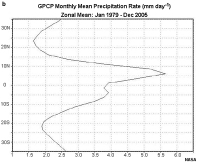
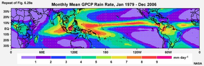
The annual mean precipitation map (Fig. 5.29a, above) indicates that the wettest regions of the tropics are the Maritime Continent, the ITCZ over the Pacific, and the Amazon. The average latitude of the ITCZ over the Atlantic and Pacific is north of the equator and it produces the peak in annual precipitation at about 7°N (Fig. 5.29b, above). Very high precipitation amounts are observed over the South Pacific Convergence Zone or SPCZ (the axis of high values extends southeastward from New Guinea, north of Australia) and the South Atlantic Convergence Zone or SACZ (axis extends southeastward from Brazil). A relative minimum occurs over central, southern Indonesia, in the middle of the wettest regions.
The driest regions are the Sahara, the Arabian Peninsula, eastern and south Pacific and the south Atlantic. These regions are located beneath the semi-permanent anticyclones.
The greatest rain accumulations in the tropics are produced by organized mesoscale systems containing both deep convective and stratiform precipitation (Fig. 5.31 a, b). Shallow convective precipitation is predominantly oceanic and outside of the heavy precipitation areas (Fig. 5.31c).
Tropical precipitation also includes snow and ice, which helps to maintain glaciers even at the equator. Tropical glaciers exist in the Andes, Himalayas, East Africa, Indonesia, and Mexico.65 Although snow and ice are a tiny fraction of tropical precipitation, glaciers are vital components of regional water cycles; they are reservoirs that maintain ground water in dry regions. Decreasing snowfall and melting due to increase in surface temperatures has led to an accelerated shrinking of tropical glaciers and raised concerns about future catastrophic droughts and floods.65
TRMM Online Visualization and Analysis System (TOVAS),
http://disc2.nascom.nasa.gov/Giovanni/tovas/
Global Outlook on Snow and Ice, Tropical Glaciers,
http://www.unep.org/geo/geo_ice/PDF/GEO_C6_B_LowRes.pdf
5.3 Precipitation »
5.3.4 Annual Precipitation »
Box 5-6 Major Influences on the Distribution of Annual Precipitation in the Tropics
Water vapor content
- Tropical oceans and the maritime continent have high precipitation amounts because of strong solar heating, evaporation, and convection.
- Continental regions are drier because they are far from the primary sources of moisture.
- Higher elevations are colder and thus have a lower saturation specific humidity.
Large-scale mechanism for lifting air to its condensation level
- The low-level convergence zones have high precipitation amounts.
- The subtropical deserts are associated with high pressure and subsidence.
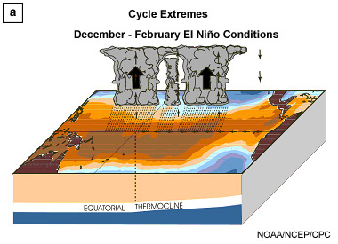
- The contrasting vertical motion between the eastern and western side of the tropical ocean contrasting vertical motion between the eastern and western side of the tropical ocean affects the distribution of precipitation. The eastern side of tropical oceans is cooler and mostly stable (dominated by subsidence inversion); cloud development is shallow; and very little precipitation occurs. The western side of tropical oceans is warmer; the troposphere is more unstable and prone to thunderstorm and heavy precipitation, except during El Niño episodes when sea surface temperatures are anomalously warm over the eastern, equatorial Pacific and a corresponding shift occurs in precipitation maximum.
Relief
- Orographic lift on the windward side of mountains enhances precipitation where prevailing winds are favorable.
- Rain shadows develop on the leeward side of mountain ranges due to adiabatic warming with descending flow.
- Mountains can serve as a barrier to low-level moisture.
Amount and type of cloud condensation nuclei
- Maritime aerosols, such as sea spray, generally enhance precipitation through warm rain processes.
- Hygroscopic or small aerosols, which are usually found over continents, tend to suppress precipitation.
The highest average annual precipitation amounts are on the windward side of tropical mountains, whereas the lowest are found far inland, in the subtropics on the western coasts where high pressure dominates, and on the leeward side of mountains. Extremes of annual precipitation are presented in a focus section at the end of the chapter.
The highest average annual precipitation amounts are on the windward side of tropical mountains, whereas the lowest are found far inland, in the subtropics on the western coasts where high pressure dominates, and on the leeward side of mountains. Extremes of annual precipitation are presented in a focus section at the end of the chapter.
5.3 Precipitation »
5.3.4 Annual Precipitation »
5.3.4.1 Variability of Annual Precipitation
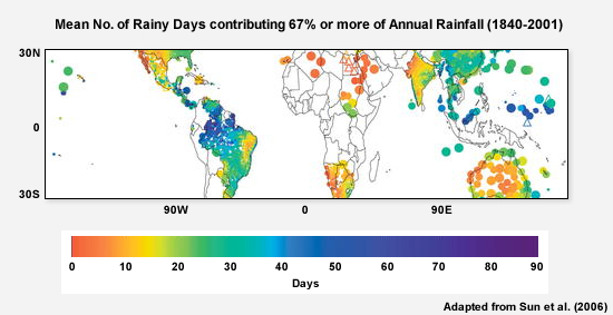
Annual precipitation amounts provide only a partial picture of tropical precipitation. We also need to know how often it rains in a given location in order to make decisions about agriculture, water resource management, and hydroelectric power generation. The variability of precipitation can be measured by counting the number of days that contribute most of the annual rainfall. Figure 5.32 shows the average number of rainy days contributing 67% of the annual precipitation for the period 1840-2001.66 Only stations with records of more than 300 days per year are shown. Precipitation frequency varies greatly from continent to continent and across some regions. A distinctive pattern of highly variable, moderately variable and least variable regions is evident.
What kind of climate is expected in the red areas? How about the blue areas? (Type your response in the box below.)
Feedback:
Red areas correspond to deserts while blue areas occur in tropical humid or wet climates. For example, in the Amazon Basin, rainfall occurs on more than 80 days whereas for most of Australia the annual precipitation falls in less than 20 days. In other semi-arid regions, such as the African Sahel and northwest India, each rainy day is critical because agriculture is a dominant sector of their economy. Populations are vulnerable to drought and famine if the rains fail or arrive later than normal. Ironically, some of the semi-arid regions are also susceptible to flash floods, since a few days of very heavy rainfall can overwhelm local watersheds.
Famine Early Warning System (FEWS) for Africa, http://www.cpc.noaa.gov/products/african_desk/
African Center of Meteorological Applications for Development (ACMAD), http://www.acmad.ne/
CILSS, Offices of the Permanent Inter-states Committee for Drought Control in the Sahel, www.cilss.bf/
5.3 Precipitation »
5.3.4 Annual Precipitation »
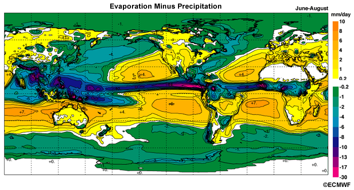
5.3.4.2 Annual Evaporation minus Precipitation
The distribution of evaporation minus precipitation (E–P) is a useful quantity for understanding variability in global and regional water balances. An increase in E–P is consistent with the beginning of a drought while a decrease in E–P indicates that a region is becoming wetter.
Annual precipitation exceeds evaporation along the ITCZ, SPCZ, in the Maritime Continent, much of South and Central America, and central Africa (Fig. 5.33)-places which receive the highest annual precipitation amounts as shown in Fig. 5.29. The Maritime Continent and Central America have the greatest net precipitation.
Over most of the tropical oceans, evaporation exceeds precipitation (Fig. 5.33). Australia is the driest continent; only a tiny part of northern Australia has more precipitation than evaporation annually. Interestingly, over the year in the Sahara Desert, evaporation is balanced by precipitation. However, the Sahel, between the Sahara and central Africa, has more evaporation than precipitation. For this region, slight variations in circulation patterns can be crucial.
Monitoring Sahel precipitation, AGRHYMET, http://www.agrhymet.ne/eng/index.html
Global Drought Monitor, http://drought.mssl.ucl.ac.uk/
US Drought Assessment,
http://www.cpc.noaa.gov/products/expert_assessment/drought_assessment.shtml
5.3 Precipitation »
5.3.5 Seasonal Precipitation
When precipitation occurs is as important as the amount of precipitation that occurs. We are interested in understanding the tropical seasonal precipitation cycle and its variability because tropical precipitation is a critical part of the global water and energy cycle. The seasonal distribution of precipitation influences how people live. Agriculture is a dominant part of many economies in the tropics and agricultural activities are controlled by the start, duration, and end of the rainy season.
The rainy season brings cooler temperatures to equatorial areasrainy season brings cooler temperatures to equatorial areas as more clouds means that more sunlight is reflected to space and thunderstorm downdrafts bring air with low equivalent potential temperature, θe, to the surface. Unfortunately, the rainy season also brings water-borne diseases, such as malaria and cholera, to many parts of the tropics. Public health concerns are not limited to the rainy season as meningitis can flourish during the dry season when dust storms are prevalent in tropical Africa and Asia.
![]() Below is an annual precipitation map (repeat of Fig. 5.29a). How do you think the pattern changes seasonally? What accounts for seasonal changes?
Below is an annual precipitation map (repeat of Fig. 5.29a). How do you think the pattern changes seasonally? What accounts for seasonal changes?
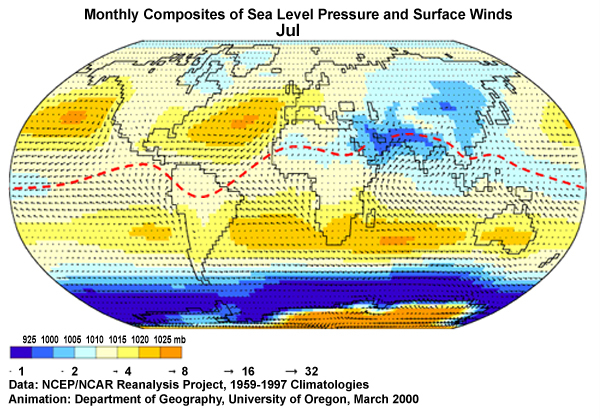
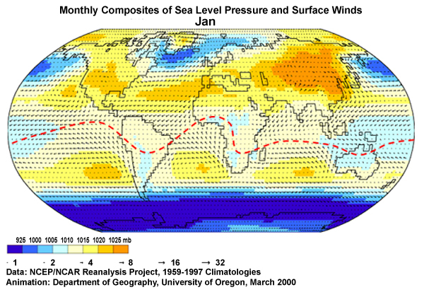
Hint: Recall the global surface pressure and wind patterns in Fig. 5.30 (Jan and Jul composites are shown below)
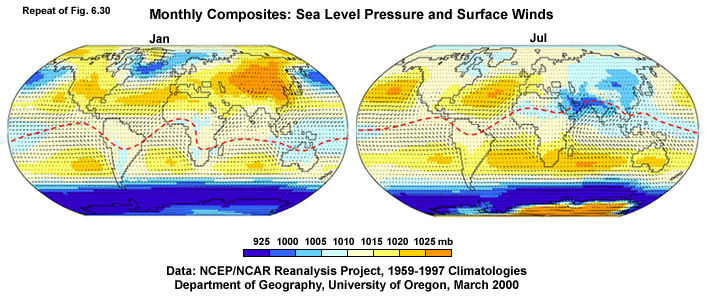
Seasonal precipitation patterns (Fig. 5.34, below) are strongly influenced by seasonal changes in quasi-stationary pressure systems, regional convergence zones, and monsoonal circulations. In general, tropical precipitation is highest during the summer and lowest during the winter.
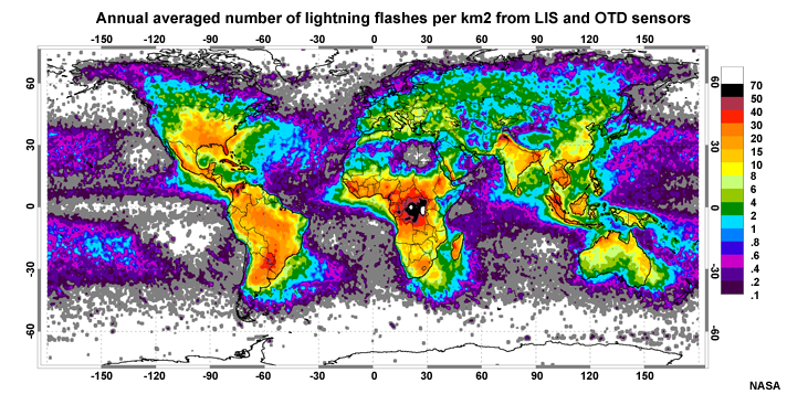
The most dramatic feature in the seasonal precipitation maps (Fig. 5.34, above) is the migration of the ITCZ. During the austral or southern hemisphere (SH) summer (January), the ITCZ extends diagonally from west to southeastern Africa yet is relatively zonal across northern Africa during the boreal or northern hemisphere (NH) summer (July). Precipitation over central Africa is much less than over other tropical continental regions despite having the maximum in lightning flash density67 (Chapter 2, Fig. 2.35) and some of the world's most intense storms.39
The July precipitation maximum, centered over the Bay of Bengal, is an outstanding feature of the boreal summer and is associated with the monsoonal circulations. During the austral summer, maximum rain rates are experienced over Madagascar as well as over and west of the Maritime Continent.
Another prominent feature of the austral summer is a band of precipitation, along the SPCZ, that extends southeastward over the south Pacific Ocean from Indonesia to about 30°S and 140°W. During the boreal summer, the SPCZ retreats eastward and northward. A relative minimum exists between the ITCZ and the SPCZ. The ITCZ remains north of the equator over the Pacific and Atlantic even during the austral summer (January).
The precipitation rate over the eastern Pacific north of the equator has a large annual range. Rates change from 11 mm day-1 in the summer to less than 3 mm day-1 in the winter. This range is comparable to that of monsoon regions, which is especially interesting since this dramatic change is happening in the absence of land/ocean heating differential.
It is not surprising that the Amazon Basin has the largest rain forest in the world when one considers that it is equatorial and ideally located downwind of easterly trade winds during the austral summer (Fig. 5.35). Warm moist air from the Atlantic fuels thunderstorms and heavy rainfall, whose rate is comparable with the Maritime Continent. The ITCZ remains over or close to equatorial South America except during July and August when the ITCZ moves to the northern part of the continent (Fig. 5.35b).
The Amazon rainforest is not only a response to seasonal rainfall but a significant source of water vapor and latent heat through evapotranspiration, which maintains the rainfall. A study of the vegetation leaf area cycle over five years has uncovered the surprising result that leaf area increases over the Amazon during the dry season71 (Fig. 5.36).
The leaf area and evapotranspiration increase during the period of little rain and abundant sunlight (Fig. 5.36). Eventually, warm, moist air triggers widespread, air mass thunderstorms. It is theorized that convergence into the initial thunderstorms starts the cross-equatorial flow that marks the onset of the next rainy season.72,73
Amazon Vegetation and the transition to the rainy season,
http://earthobservatory.nasa.gov/Study/AmazonLAI/printall.php
5.3 Precipitation »
5.3.5 Seasonal Precipitation »
Box 5-7 The ITCZ Position
Why do you think that the ITCZ remains north of the equator over the Pacific and Atlantic even during austral summer? (Type your response in the box below.)
Feedback:
The reasons are not simple.68,69 The underlying causes are the asymmetric distribution of land between the NH and SH as well as the orientation of land along the eastern boundaries of the oceans. The position of the ITCZ over the Pacific and Atlantic is a result of a coupled ocean-atmosphere response system. We need to consider the annual cycle of the ITCZ relative to the narrow area of relatively cool SSTs (the cold tongue) and the surface winds along the equator.
Let us examine the case of the ITCZ over the Pacific. The eastern equatorial Pacific has strong upwelling where the trade winds stress pulls surface waters towards the west. Along the equator, upwelling occurs where ocean currents diverge because of the directional switch of the Coriolis effect. Therefore, a cold tongue extends from the eastern to central Pacific along the equator. Convection is inhibited and so the ITCZ does not form at the equator. It could form on either side of the cold tongue. Why then does it form to the north? The ITCZ forms north of equator where the SSTs are higher. How does the SST become warmer to the north or how does the SST become relatively cooler to the south? Numerical models of the annual cycle with an aqua planet produce symmetric circulations. The indications are that the presence and orientation of the eastern continental boundary introduces asymmetries in the trade wind velocity, which, in turn influences the coastal upwelling leading to warming north of the equator and cooling to the south. Southerly trade winds cross the equator and converge with the northeast trades where SSTs are warmer, leading to rising motion and precipitation.
It is also hypothesized that stratus clouds, which are common along the eastern boundaries of the tropical oceans (Fig. 5.13), increase the reflection of sunlight. Enhanced reflection cools the surface and strengthens the cross-equatorial temperature gradient and convergence to the north of the equator.70
A coupled atmosphere-ocean feedback also occurs in the Atlantic but on a smaller scale.
5.3 Precipitation »
5.3.5 Seasonal precipitation »
5.3.5.1 Seasonal Evaporation minus Precipitation (E-P)
The seasonal distribution of E-P (Fig. 5.37) differs from the annual mean in a similar fashion as the seasonal precipitation differs from the annual precipitation. The eastward extension of the SPCZ is fairly prominent in December to February and the ITCZ locations are similar. Other outstanding features are broad regions along the western side of the oceans, where precipitation exceeds evaporation during the summer. During June to August, the area of excess precipitation is proportionally wider in the Pacific than the Atlantic.
Examine the figures below. What do you think causes excess precipitation over western oceans in June to August? (Type your response in the box below.)
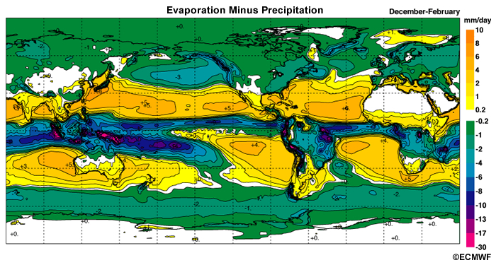
Feedback:
Warmer SSTs occur over the western ocean boundaries and cool upwelling occurs along the eastern boundaries in response to the prevailing trade winds. During the NH winter, E-P is a maximum along the western ocean because dry, cold air moves from the continents across the warm ocean leading to very high evaporation rates (Fig. 5.4). During the NH summer, the air-sea contrasts in temperature and humidity are reduced over the warm ocean currents leading to less evaporation. A broader area of excess precipitation exists across the Pacific because of its larger region of warm SSTs, compared with the Atlantic. The south Atlantic E-P magnitude and area are much smaller than the north Pacific and Atlantic.
5.3 Precipitation »
5.3.5 Seasonal Precipitation »
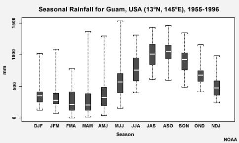
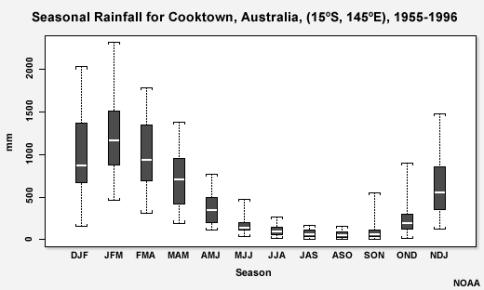
5.3.5.2 Seasonal Precipitation in West and Central Pacific
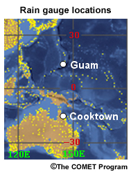
The solar declination angle is the dominant factor in the seasonal precipitation cycle, as illustrated in Guam and Cooktown (Australia), where the peak in the precipitation follows the maximum insolation period (Fig. 5.38). The monthly precipitation totals are highly variable for Cooktown during December to March. This variability may be due to the influence of the El Niño-Southern Oscillation (ENSO) cycle, whose anomalies are usually maximized during the same period.
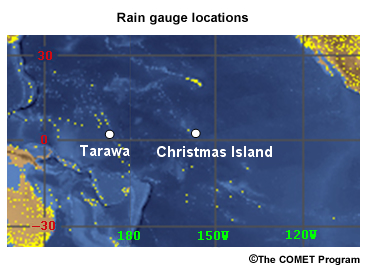
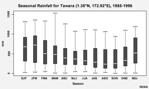
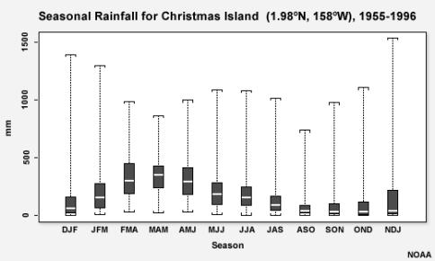
For stations close to the equator, the seasonal variability of rainfall is small. However, the amount of rainfall can still vary dramatically by location. For example, at Tawara (~1.5°N, 172°E), the average seasonal precipitation is about five times that of Christmas Island (~2°N, 158°W) (Fig. 5.39). At Tawara, the ITCZ is close to the equator while to the east, the mean ITCZ position is north of the equator. Christmas Island is located in the equatorial dry zone that is associated with the cold tongue of equatorial waters extending from the eastern to central Pacific. The influence of ENSO is also contributing to the extreme variability seen in the monthly totals for Christmas Island compared with Tawara. The variability is maximized during the winter months. During El Niño winters, precipitation increases over the central and eastern Pacific thereby dramatically increasing precipitation over Christmas Island.
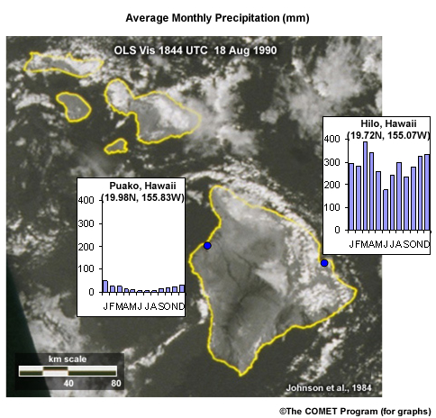
The impact of topography on precipitation is illustrated by the differences in precipitation received on the windward and leeward sides of the Hawaiian Islands (Fig. 5.40).
5.3 Precipitation »
5.3.5 Seasonal Precipitation »
5.3.5.3 Seasonal Precipitation in West Africa
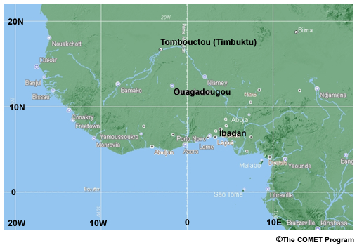
Based on what you have learned about the factors that influence annual and seasonal precipitation amounts, how do you think rainfall amounts will vary from Ibadan to Tombouctou (Timbuktu)? (Type your response in the box below.)
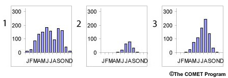
Try to match the following monthly average precipitation graphs (1, 2, 3) with the correct cities (above).
Feedback:
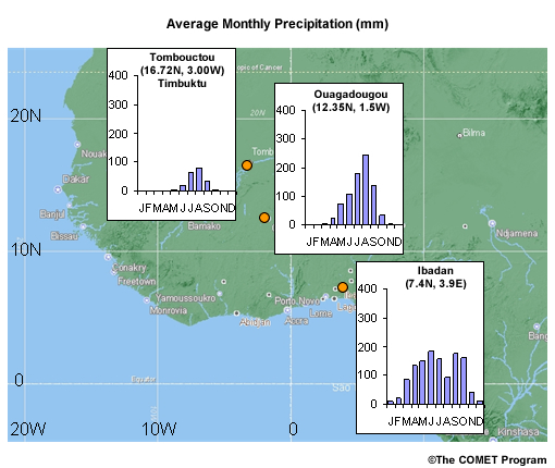
In general, precipitation amounts decrease with latitude and distance from the ocean (Fig. 5.41). All three stations have minimum precipitation in the winter months and most of their precipitation in the summer months. Ibadan is the only one of the three cities that receives more than 10mm of precipitation in each month. Tombouctou (Timbuktu) is on the edge of the Sahara Desert. These areas receive precipitation only in the summer when strong solar heating of the surface leads to rising motion, low pressure, and the inflow of moist air from the ocean and equatorial Africa.
Apart from the change in the amount of precipitation, do you notice any other differences in the seasonal rainfall patterns of Tomboutou and Ibadan? (Type your response in the box below.)
Feedback:
There are two maxima in the monthly rainfall at Ibadan.
Why do you think these two maxima occur? (Type your response in the box below.)
Feedback:
The two peaks are associated with the semi-annual passage of the ITCZ. The July minimum is also influenced by seasonal shifts in atmospheric circulation and SSTs. July and August are the peak months of the monsoon. During the monsoon, southwesterly flow brings cool air from the ocean over the warm continent, which leads to lower relative humidity and less precipitation.
5.3 Precipitation »
5.3.5 Seasonal Precipitation »
5.3.5.4 Seasonal Precipitation in the Indian Subcontinent
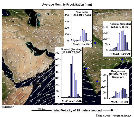
Seasonal precipitation in the Indian subcontinent is controlled by the monsoonmonsoon. Most of the precipitation falls between May and October (Fig. 5.42). Not surprisingly some of the highest precipitation totals in the world are recorded along the western coast of India, e.g., Mumbai. The heavy precipitation results from a strong onshore flow of moist air from the ocean being lifted by the terrain in a region of surplus radiational heating. Kolkata (Calcutta) also receives abundant precipitation due to moist air from the Bay of Bengal. Inland areas such as New Delhi and Bengalooru (Bangalore) receive less precipitation.
5.3 Precipitation »
5.3.5 Seasonal Precipitation »
5.3.5.5 Seasonal Precipitation in the Americas
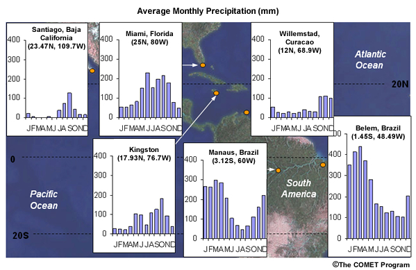
Like elsewhere, precipitation in the Americas (Fig. 5.43) is influenced by the seasonal cycle, the ITCZ, topography, and distance from the ocean. Manuas, Brazil has dual maxima in seasonal precipitation associated with the ITCZ migration cycle (Fig. 5.35). During both summer and winter, Manuas lies within a region of confluence. Although Belem and Manuas are similar in latitude, Belem, which is near the coast, receives more precipitation and has a single peak during the austral summer. During the winter Belem is located in prevailing southeasterly flow which is cooler and less moist.
In Kingston, Jamaica, the May-June rainy season is associated with heating due to the maximum solar declination angle but the later rainy season is not. Between September and November, SSTs in the western Caribbean are at their maximum and the island is affected by tropical waves, depressions, and tropical cyclones. A minimum in rainfall occurs over the western Caribbean and Central America in July.75,76 The mid-summer rainfall minimum is associated with a relative maximum in sea level pressure, cool SST anomalies, and a maximum at 925 hPa known as the Caribbean Low-level Jet or CLLJ.77,78 The stronger wind mixes the warm surface waters with cooler water from below, lowering the SST. Sea level pressure increases in July when the North Atlantic High is farthest west and south. In addition, the stronger CLLJ in the mid-summer leads to a reduction in the SSTs over the southern Caribbean and a stronger meridional SST gradient across the region.78 Divergence in the entrance region of the CLLJ is one of reasons for low precipitation over northern Venezuela and the southeastern Caribbean.78 The islands in the southern Caribbean, e.g. Curacao, are far south of the regular summer storm tracks and are under the influence of offshore winds from the continent. They receive their maximum precipitation during November to December when the ITCZ shifts towards the south and prevailing northeasterly winds bring a constant supply of warm oceanic air into the region.
In Kingston, Jamaica, the May-June rainy season is associated with heating due to the maximum solar declination angle but the later rainy season is not. Between September and November, SSTs in the western Caribbean are at their maximum and the island is affected by tropical waves, depressions, and tropical cyclones. A minimum in rainfall occurs over the western Caribbean and Central America in July.75,76 The mid-summer rainfall minimum is associated with a relative maximum in sea level pressure, cool SST anomalies, and a maximum at 925 hPa known as the Caribbean Low-level Jet or CLLJ.77,78 The stronger wind mixes the warm surface waters with cooler water from below, lowering the SST. Sea level pressure increases in July when the North Atlantic High is farthest west and south. In addition, the stronger CLLJ in the mid-summer leads to a reduction in the SSTs over the southern Caribbean and a stronger meridional SST gradient across the region.78 Divergence in the entrance region of the CLLJ is one of reasons for low precipitation over northern Venezuela and the southeastern Caribbean.78 The islands in the southern Caribbean, e.g. Curacao, are far south of the regular summer storm tracks and are under the influence of offshore winds from the continent. They receive their maximum precipitation during November to December when the ITCZ shifts towards the south and prevailing northeasterly winds bring a constant supply of warm oceanic air into the region.
Although close in latitude, Miami, Florida and Santiago, Mexico, in Baja California, have very different precipitation records. Miami has precipitation all year with a peak during the summer months. Precipitation remains high during the fall because of tropical disturbances (waves, depressions, and cyclones). During the winter, Miami is also affected by mid-latitude weather systems. Santiago is on the west coast where the ocean is much colder due to upwelling and less moisture is available for precipitation. Its peak in late summer is mainly associated with the passage of tropical disturbances.
5.3 Precipitation »
5.3.6 Intraseasonal Tropical Precipitation
Strong variability in the intensity and distribution of tropical precipitation also occurs at sub-seasonal time scales. Tropical precipitation fluctuates over a 30-60 day cycle known as the 'Madden-Julian Oscillation (MJO)', 79 '30-60 day oscillation', and '30-60 day wave'.
Strong variability in the intensity and distribution of tropical precipitation also occurs at sub-seasonal time scales. Tropical precipitation fluctuates over a 30-60 day cycle known as the 'Madden-Julian Oscillation'79 or 'MJO', '30-60 day oscillation', and '30-60 day wave'.
The MJO is marked by large regions of enhanced and suppressed precipitation moving eastward across the tropics and is most prominent over the Indian and Pacific Oceans. Anomalously high rainfall is usually apparent first over the western Indian Ocean, and remains evident as it moves over the very warm western and central tropical Pacific Ocean. This pattern of tropical rainfall generally becomes less distinct as it moves over the cooler waters of the eastern Pacific but then reappears over the tropical Atlantic, Africa, and Indian Ocean. .
The MJO is monitored primarily with satellite data such as the Outgoing Longwave Radiation or OLR (a measure of tropical convection and rainfall). Radiosonde data are used to assess the thermodynamic and dynamic changes associated with the MJO passage in order to improve their prediction. Better forecasts of the MJO are needed because the MJO favors tropical cyclone formation where it enhances rising motion over warm oceans or it inhibits formation during its subsidence phase. The MJO also influences midlatitude weather especially in the winter. For example, plumes of moisture flowing from MJO rainfall maxima over the central Pacific lead to heavy precipitation and floods along the west coast of the United States. You can explore more about the MJO in the COMET webcast The Madden-Julian Oscillation Life Cycle (http://www.meted.ucar.edu/climate/mjo/) presented by Dr. Roland Madden.
Tropical precipitation is also modulated by equatorial waves that move more quickly than the MJO. Intra-seasonal tropical variability is examined in detail in Chapter 4.
Tropical precipitation is also modulated by equatorial waves that move more quickly than the MJO. Intra-seasonal tropical variability is examined in detail in Chapter 4.
http://www.cpc.noaa.gov/products/intraseasonal/
Daily MJO Indices,
http://www.cpc.noaa.gov/products/precip/CWlink/daily_mjo_index/mjo_index.html
5.3 Precipitation »
5.3.7 Diurnal Cycle of Precipitation in the Tropics
![]() At what time of day does it rain the most in the tropics?
At what time of day does it rain the most in the tropics?
The instinctive response would favor the afternoon-the period of maximum heating and maximum boundary layer depth. However, the diurnal cycle of precipitation is influenced by other factors such as surface properties (land or ocean), topographically-induced circulations (e.g., sea/land breezes), and propagating MCSs.80
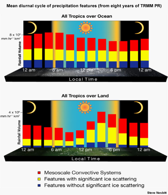
On average, a small but significant rain maximum occurs over the tropical oceans during the pre-dawn hours80 (Fig. 5.44a). Over land, total maximum rainfall occurs during the afternoon but rainfall from MCSs peaks after midnight (Fig. 5.44b). The diurnal variability is more pronounced over land. Oceanic rainfall volume is controlled mostly by variations in the number (and total areal coverage) of MCSs,80 which is in turn strongly influenced by large-scale periodic events like the MJO.
A number of explanations have been given for the early morning maximum and afternoon minimum in oceanic precipitation and the reasons are still being debated. One explanation is that heating differences between convection and surrounding air causes a daily variation in the divergence of the winds which modulates the convection.81 Another study proposes that during the afternoon, the tops of the oceanic cloud absorb sunlight which increases the static stability of the clouds and leads to less active convection and less precipitation.82 At night, the tops of oceanic clouds are losing heat faster, leading to more instability, and precipitation increases. A third factor may be that at night, loss of heat by longwave radiation increases the relative humidity, which favors cloud development.83
5.3 Precipitation »
5.3.7 Diurnal Cycle of Precipitation in the Tropics »
5.3.7.1 Seasonal Variations in Tropical Rainfall Diurnal Cycles
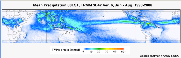
The diurnal patterns in all seasons are modulated by the position of the ITCZ and the low-level flow relative to significant topographic gradients (high terrain or coast lines). During the boreal summer (Fig. 5.45a, above), early-morning maximum rainfall is found over oceanic, near-coastal regions such as Guinea West Africa, the Isthmus of Panama, and west of the Indian and Indochinese peninsulas (Fig. 5.45a). Through the morning, coastal rain areas increase but rainfall over land decreases to its minimum. The daily peak intensity over land occurs in the afternoon over land areas such as northern tropical Africa, Central America, the Philippines, and Indochina. Rainfall decreases in intensity but the rain areas continue to expand to a maximum near midnight. Over the Amazon, peak intensity occurs near midnight. After midnight, intensity diminishes but broad areas of rainfall remain and the peak intensities are found over the ocean and coasts. Maxima in oceanic rainfall intensity are found in the Bay of Bengal, the ITCZ over the East Pacific, and in the SPCZ east of Papua New Guinea. Hourly precipitation rates in the eastern Pacific and eastern Atlantic are the highest of any season.
Sea and land breezes help to trigger convection that often interacts with complex terrain and other sources of convection to produce diurnally modulated systems. For example, over northern South America the minimum daily precipitation is generally found between 0900 and 1100 LT. However, strong orographic effects are produced by the three branches of the Andes (oriented in a north-south direction) with elevation exceeding 5000 m. An afternoon to evening peak is found over northwestern slopes and the northern coast due to solar thermal heating and orographic lift of onshore low-level moisture from the Pacific and the Caribbean, respectively. On the western side of the central Andes, maxima are observed during the afternoon and near midnight. On the eastern side of the Andes, maximum precipitation occurs near midnight due to MCSs propagating inland from the east coast.
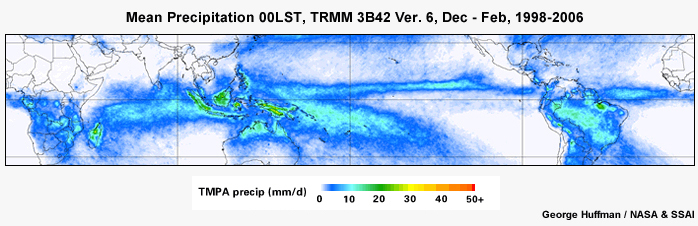
During the austral summer (Fig. 5.45b, above), the diurnal cycle is modulated by the north-south shift in the ITCZ over Africa. Precipitation rates are highest over Madagascar, Indonesia, and South America during the evening to nighttime hours. South America has two large regions that receive heavy precipitation daily; one over the Amazon basin, which reaches maximum during the late afternoon and a less intense maximum to the south during the nighttime to early morning. The latter is dominated by the lifecycle of MCSs which initiate in the foothills of the Andes in the evening, intensify, and expand while moving to the east.
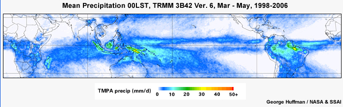
The March-May equatorial transition (Fig. 5.45c, above) is unique in having dual ITCZs across the Pacific with the stronger branch in the NH. Maximum precipitation intensity and areal extent in the Pacific ITCZs occurs between 05 and 07 LST and the minimum between 19 and 22 LST. Continental precipitation is most intense near the Amazon estuary and Indonesian maritime continent between 18 and 22 LST. In the Amazon, precipitation moves from the coast towards the southwest during the day; inland precipitation expands between 12 and 20 LST and shrinks to a minimum at 11 LST. In the maritime continent the island topography greatly influences the diurnal cycle. During late morning, precipitation is a minimum over the islands and a maximum over the neighboring ocean. In central Africa, the heaviest precipitation outlines the East African Mountains and Lake Victoria in the late afternoon and early evening. Continental precipitation moves westward and begins diminishing in the morning to its daily minimum between 10 and 11 LST. The sea-land breeze effect is also evident along the west African coast near the equator.
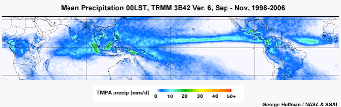
The daily precipitation cycle during September-November (Fig. 5.45d, above) is similar to other seasons. A unique feature of this season is that precipitation rates in the ITCZ across the central Pacific during September-November are the highest of all seasons. With the large-scale precipitation farther north, the daily precipitation maxima shifts to northern Indonesia, the Gulf of Panama, and western Amazonia.
The diurnal patterns in all seasons are modulated by the position of the ITCZ and the low-level flow relative to significant topographic gradients (high terrain or coast lines).
5.3 Precipitation »
5.3.7 Diurnal Cycle of Precipitation in the Tropics »
5.3.7.2 Regional Patterns of Tropical Rainfall Diurnal Cycles
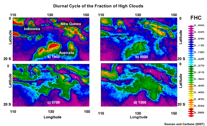
Over Australia and Indonesia, the daily cycle of deep convection and, by association, precipitation, is influenced significantly by topography84 (Fig 5.46). In the evening (1900 LT), precipitation is heaviest over land and at a minimum over the ocean and along the coasts. Over Papua New Guinea, maximum precipitation occurs along the slopes of the central mountain range (in bands on the northern and southern sides of the mountainous backbone) during early evening and nighttime (0000 LT). In contrast, during the early morning (0700 LT), precipitation is heaviest over the ocean and along the coastlines, and at a minimum over the land. IR brightness temperatures are useful for examining the diurnal cycle because tropical cold cloud tops are usually associated with thunderstorms and images are available every 15-30 minutes. However, the IR precipitation estimates do not include precipitation from warm clouds and can overestimate precipitation in the late stage of MCS lifecycle when thick cirrus can be misidentified as precipitation.
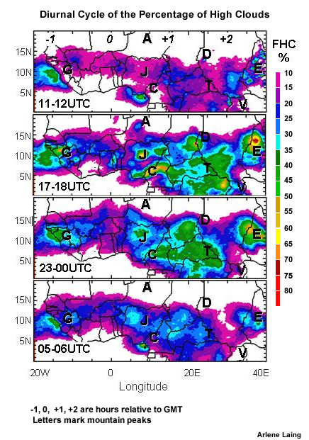
For northern Tropical Africa, we examine the distribution of cold clouds, which serve as a proxy for precipitation from thunderstorms85 (Fig. 5.47). Over the land, the peak in overall intensity and area of precipitation occurs during the late afternoon to evening (1700-1800 UTC) and the minimum occurs one or two hours before noon. Along the coast, precipitation is at a maximum in the morning. The daily cycle of precipitation is also influenced by topography. The highest frequency of intense convection occurs over or to the west of high terrain. Convection starts as elevated terrain is heated and air flows upward along the slopes. The convection grows and is steered westward by the prevailing winds. During the late afternoon to early nighttime hours, the convection is more intense (1700-1800 UTC). As MCSs reach the mature stage of their lifecycle, a broad stratiform region develops and peaks near midnight (2300-0000 UTC). The intensity of the precipitation decreases but the area of rainfall is maintained through the nighttime (0500-0600 UTC).
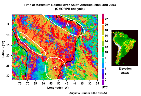
The time of maximum rainfall over South America (Fig. 5.48) is strongly influenced by the topography and prevailing winds. The sea-breeze effect is evident over northeastern South America (region A, Fig. 5.48) where the period of maximum precipitation shifts southwestward inland from the coast (from noon to about 0600 LT). The period of maximum rain frequency shifts as squall lines shift southwestward with time. Precipitation in the western Amazon basin is influenced by mountain breeze circulations due to the Andes Mountains (region B, Fig. 5.48). Systems over the Amazon are fueled by moist air from the Atlantic and local evapotranspiration from the rainforests.71 Shallow convection produces about 10% of precipitation in the Amazon basin.86 In the south, mesoscale convective systems are fueled by a ribbon of warm, moist air from the Amazon. The precipitation cycle south of 20°S is mostly influenced by propagating MCSs which last through the nighttime hours. These MCSs initiate along the high terrain and move east (region C in Fig. 5.48).
5.3 Precipitation »
5.3.8 Interannual Variability of Tropical Precipitation
Precipitation is sensitive to small spatial and temporal variations in the general circulation. Fig. 5.49 illustrates the temporal variability of the monthly precipitation anomaly across the tropics (35°S-35°N) from the TRMM data and from 21 gauge sites. Dramatic swings from anomalously low to high precipitation rates can occur in one year, as occurred between the strong El Niño of 1997-98 and the La Niña of 1998-99.
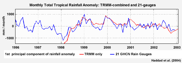
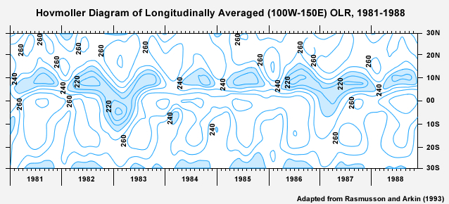
Interannual variability of the mean latitudes of precipitation is evident in Fig. 5.50, an eight-year time series of the zonal mean outgoing longwave radiation, which can be considered a proxy for convective precipitation86. Dramatic shifts are seen during the El Niño episodes of 1982-83 and 1987. Interannual shifts in circulation centers can inflict tremendous harm on populations in the tropics. For example, the African Sahel experiences devastating droughts when the ITCZ does not migrate as far north as normal.
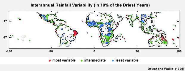
Interannual variability can also be measured by how much of the annual rainfall is expected in the 10% of the years that are driest or the 0.1 quantile.89 Figure 5.51 shows the geographic patterns of interannual variability of precipitation. Notable areas include:
- Northeast Brazil, which has long been documented as having one of the most variable climates, with frequent droughts.
- Northeastern Australia, where the strong connection to ENSO makes it more variable than areas with comparable mean annual rainfall.
- Coastal Ecuador and Peru, where El Niño brings extreme heavy precipitation and La Niña periods are relatively dry.
- Southeastern and east African coast, where many factors contribute to variability including ENSO.90 Although the 1997-98 El Niño was relatively wet for Mozambique, about two-thirds of El Niño periods since 1950 were dry.91 Variability in the Indian Ocean SSTs is likely to be more dominant than ENSO. Anomalous warm SSTs during 1997-98 produced strong convection over eastern Africa and a 20-160% increase in rainfall in the Lake Victoria region, where as previous El Niño periods caused a 15-25% increase in rainfall.92 Below-normal southwest monsoon flow is associated with less upwelling, leading to above normal SSTs over the North Indian Ocean and the Arabian Sea. East African rainfall variability is influenced to a lesser extent by the eastern and tropical areas of the Atlantic93 and mid-latitude circulations over the eastern Mediterranean and the Arabian peninsula, specifically, anomalies in the 500 hPa geopotential height.94
- Northwestern India, where large variability is likely to due to the position of the monsoon trough and anomalies in the Indian Ocean SSTs.
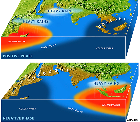
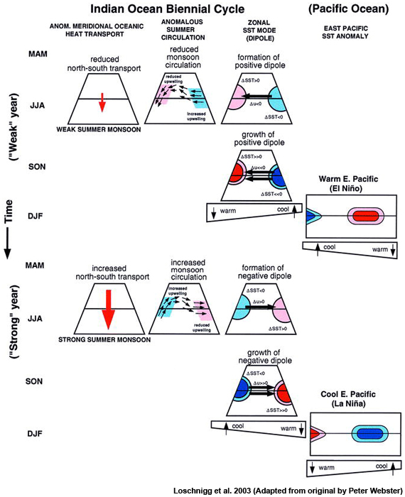
Regions with low interannual variability of precipitation include:
- Central and West Africa and a small area of South Africa
- Amazon Basin and interior of tropical South America
- Indochinese peninsular and inland southern China
- Mountains of Mexico
All other areas experience intermediate variability in annual precipitation. It should be noted that not all areas of high variability are responses to ENSO. Climate scientists are examining stratospheric wind reversals, anomalous Atlantic Ocean temperatures, and other factors that may cause interannual variability in precipitation across the tropics.
Reducing the Impact of Environmental Emergencies through Early Warning and Preparedness:
The Case of the 1997-98 El Niño, http://www.ccb.ucar.edu/un/index.html
Principal component analysis,
http://www.elderlab.yorku.ca/~vida/ppt/PCA.ppt
Focus Areas
Focus Areas »
Focus 1: Extremes of Tropical Precipitation
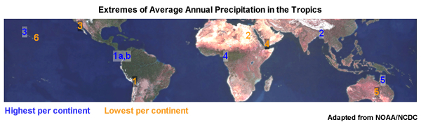
The highest average annual precipitation amounts occur:
- near oceans
- where onshore winds are prevalent
- on the windward side of tropical mountains
The lowest average annual precipitation amounts occur:
- inland, away from moisture sources
- in the subtropics, on the western coasts where high pressure dominates and specific humidity is low due to cold upwelling
- on the leeward side of mountains
| Continent | Highest Avg. (mm) |
Place | Elevation (m) |
Years of Record |
| 1a South America | 13299 ! ^ | Lloro, Colombia | 158.5* | 29 |
| 2 Asia | 11872 ! | Mawsynram, India | 1401.2 | 38 |
| 3 Oceania | 11684 ! | Mt. Waialeale, Kauai, HI | 1569.1 | 30 |
| 4 Africa | 10287 | Debundscha, Cameroon | 9.1 | 32 |
| 1b South America | 8992 ^ | Quibdo, Colombia | 36.6 | 16 |
| 5 Australia | 8636 | Bellenden Ker, Queensland | 1555.1 | 9 |
| Adapted from NOAA National Climatic Data Center (NCDC) ! The value given is the continent's highest and, possibly, the world's depending on measurement practices, procedures, and period of record variations. ^ The official greatest average annual precipitation for South America is 8991.6 mm at Quibdo, Colombia. The 13299 mm average at Lloro, Colombia [22.5 km SE and at a higher elevation than Quibdo] is an estimated amount. * Approximate elevation |
||||
| Continent | Lowest Avg. (mm) |
Place | Elevation (m) |
Years of Record |
| 1 South America | 0.8 | Arica, Chile | 29 | 59 |
| 2 Africa | < 2.54 | Wadi Halfa, Sudan | 125 | 39 |
| 3 North America | 30.5 | Batagues, Mexico | 4.9 | 14> |
| 4 Asia | 45.7 | Aden, Yemen | 6.7 | 50 |
| 5 Australia | 102.9 | Mulka (Troudaninna), South Australia |
48.8* | 42 |
| 6 Oceania | 226.8 | Puako, Hawaii, HI | 1.5 | 13 |
| Adapted from NOAA/NCDC. Sources: The first, "Climates of the World", is an NCDC publication that lists global average temperature and precipitation information for particular locations, with highlighted global extremes. The second publication is the updated "Weather and Climate Extremes" (TEC-0099) published by the US Army Corps of Engineers. The report lists global extremes for various climatological parameters and presents global map inserts as well. |
||||
NOAA National Climatic Data Center(NCDC) Extreme Weather and Climate Events,
http://www.ncdc.noaa.gov/oa/climate/severeweather/extremes.html
Focus Areas »
Focus 2: Seasonal Precipitation in Central Africa
Here we focus on the annual cycle of precipitation in Central Africa, a region that is one of the primary heat sources for the global energy cycle and where the seasonal variability of precipitation has a large socio-economic impact. As noted in Section 5.3, precipitation is influenced by several factors including, but not limited to, elevation (Fig. 5F2.1), prevailing ocean flow and circulations (Fig. 5F2.1), and low-level convergence zones (Fig. 5F2.2).
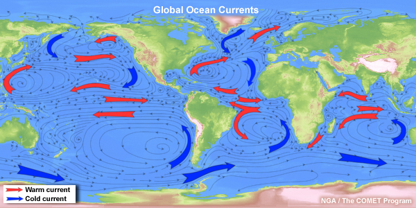
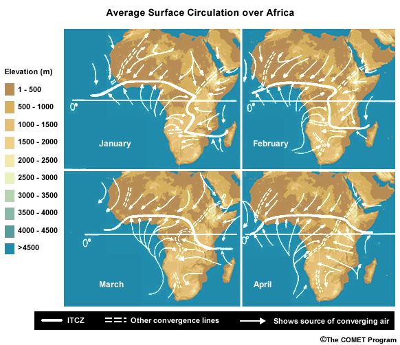
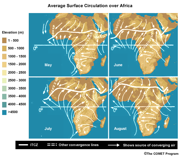
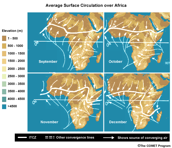
Match the graphs with the correct cities on the map. Is the trend what you expected based on information from Section 5.3.5? What do you think is influencing the trend in precipitation? (Type your response in the box below.)
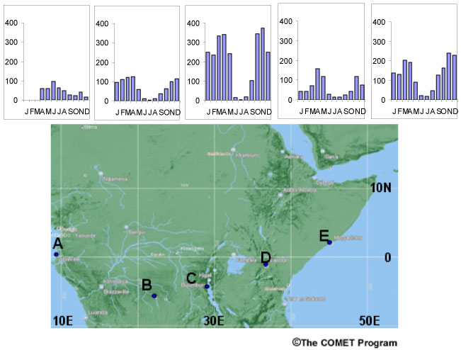
Feedback:
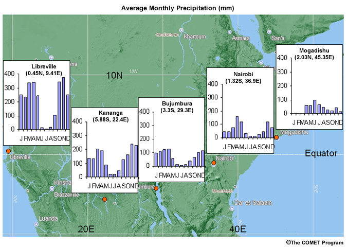
Is the trend what you expected, based on influences described in Section 5.3.4? What do you think are the major influences on the trend in precipitation in Central Africa? (Type your response in the box below.)
Feedback:
The trend is increasing precipitation towards the west (Fig. 5F2.3). Although distance from the warmer ocean is one of the influences on the amount of precipitation, in this case the major factors are the seasonal cycle and the location of the ITCZ (Fig. 5F2.2). From November through March, the ITCZ is tilted from west to southeast Africa and away from East Africa.
The shift in the ITCZ and the quasi-permanent convergence zones over the Congo Basin enhance rainfall over the west and central areas, while reducing rainfall in the east. Along the west coast, onshore monsoonal flow brings abundant moisture during the autumn and spring. In Libreville, the precipitation pattern is nearly symmetric about the summer minimum. The precipitation drops dramatically when the ITCZ is in its far north position but never completely ceases. During the austral summer, the ITCZ is never far enough south for the precipitation to have as dramatic an impact on the precipitation.
Although the prevailing winds are onshore between November and March, the Somali coast near Mogadishu is under the influence of a ridge, which suppresses precipitation. During the boreal summer, surface warming and low-level moisture carried by the Somali Jet produce the annual peak in rainfall.
The inland plateau regions have lower amounts of moisture and precipitation because of distance from the coast and the high elevation. Note that the highest peaks of East Africa are snow-covered, although the amount of snow has declined dramatically during the past two decades. Although far inland, Bujumbura has rainfall in all months because it is on the shores of Lake Tanganika.
Inter-annual variations to this seasonal precipitation pattern are related to ENSO and SST anomalies in the Indian Ocean (Section 5.3.8).
Inter-annual variations to this seasonal precipitation pattern are related to ENSO and SST anomalies in the Indian Ocean (Section 5.3.8).
Focus Areas »
Operational Focus
Water Vapor
- Saturation in the atmosphere
- When do you expect high evaporation rates?
- Factors that influence evapotranspiration rate
- Climatology of surface relative humidity in the tropics
- Climatology of surface specific humidity in the tropics
Thermodynamic Properties of Dry and Moist Air
- Using equivalent potential temperature to forecast heavy precipitation
- Thermodynamic or static energy and its application to tropical weather analysis
- Profiles of moist static energy as indicators of fair weather, isolated showers, or widespread thunderstorms with heavy rainfall
- Static energy changes with the passage of a tropical squall line
- Impact of Saharan Air Layer on vertical distribution of moisture
- Compare the vertical distribution of moisture in different regions of the tropics
Tropical Convection
- Cumulus convection, CAPE, and vertical velocity
- Convective and stratiform precipitation in tropical MCSs
- Lifecycle of a tropical squall line with trailing stratiform region
- Average convective and stratiform rain rates in the tropics
Tropical Precipitation
- Estimating tropical precipitation
- What happens to precipitation when clouds ingest smoke or other industrial aerosols
- The Madden-Julian Oscillation (MJO)
- Major factors that influence seasonal and annual precipitation across the tropics
Seasonal Precipitation
- Seasonal precipitation in West and Central Pacific
- Seasonal precipitation in West Africa
- Seasonal precipitation in Central Africa
- Seasonal precipitation in the Indian subcontinent
- Seasonal precipitation in the tropical Americas
Diurnal Cycle of Precipitation in the Tropics
- Diurnal Cycle of Precipitation in Dec-Feb
- Diurnal Cycle of Precipitation in Mar-May
- Diurnal Cycle of Precipitation in Jun-Aug
- Diurnal Cycle of Precipitation in Sep-Nov
- Diurnal Cycle of Precipitation in Australia and New Guinea
- Diurnal Cycle of Precipitation in Northern, Tropical Africa
- Diurnal Cycle of Precipitation in South America
Summary
In this chapter we explored the properties and distribution of water vapor, clouds, and precipitation in the tropics. Most of the moisture in the tropical atmosphere begins as evaporation from the tropical oceans. While the relative amount of global moisture from evapotranspiration is small, variability in those amounts is critical for semi-arid regions such as the Sahel. Furthermore, the buildup of evapotranspiration from the Amazon Basin during the dry season helps to trigger the first thunderstorms of the rainy season.
Thermodynamic or static energy is at its minimum in the middle troposphere. An increase in thermodynamic or static energy in the middle troposphere is correlated with an increase in precipitation and intensity of convection. This characteristic can be used to distinguish fair weather or undisturbed environments from environments that are conducive to thunderstorms and heavy precipitation as well as differentiate between the leading convective edge and the wake of tropical squall lines.
Tropical clouds are mostly shallow cumulus, stratocumulus, cumulus congestus, and cumulonimbus. The typical distribution of these clouds is from shallow to deep when traveling from the subtropics to the ITCZ over the ocean. A similar trend occurs from the trade inversion over the eastern side of the ocean to the west. The highest fractional cloud amounts are within the ITCZ, Asian monsoon region, and the stratocumulus layer in the subtropics, while the lowest fractional cloud amounts are in the subtropical highs. Stratiform precipitation has a greater areal coverage across the tropics but the accumulated tropical precipitation is mostly convective. In general, oceanic aerosols are fewer and larger than continental aerosols, therefore marine cumulus and stratocumulus tend to have fewer, larger drops, and lower reflectivity than clouds with continental aerosols.
Most of the precipitation falls in the summer time but regional variations are influenced by shifts in the orientation of the ITCZ, topography, convergence zones, and the passage of tropical disturbances. Over the ocean, the diurnal maximum of precipitation occurs in the pre-dawn hours and minimum occurs during the mid-afternoon. Precipitation over land reaches its daily maximum in the late afternoon, after the period of maximum heating. However, regional exceptions occur because of complex terrain, sea/land breeze circulation, and propagating mesoscale convective systems.
Places where precipitation falls in only a few months, such as parts of Australia and the Indian subcontinent, are vulnerable to droughts and related agricultural failure. The spatial and temporal distribution of moisture varies from year to year; regional variability is most dramatic during strong ENSO episodes. Continued improvement in the observation and prediction of tropical moisture and precipitation is critical to (i) our understanding of the global water and energy cycle and (ii) better quality of life in tropical countries.
Questions for Review
- Give at least three reasons why water vapor is important to weather and climate in the tropics.
- Describe at least three factors that influence the rate of evaporation and evapotranspiration.
- Give at least two reasons why there is an evaporation minimum at the equator over the tropical oceans when solar radiation per unit area is at a maximum.
- Where over the tropical oceans are the highest amounts of water vapor and where are the lowest?
- Why is the relative humidity very high over the eastern tropical ocean basins?
- Why is the equivalent potential temperature a more a useful parameter than temperature for understanding the thermodynamic structure of the atmosphere?
- Describe the basic process of convection associated with a cumulus cloud (from an air parcel being heated at the surface, to its highest level of ascent, and return to the surface).
- What is the typical distribution of cloud types and cloud depths from the subtropics to the equator?
- Why are stratocumuli prevalent over the eastern tropical and subtropical oceans?
- Define the dry static energy and the moist static energy.
- How does the vertical distribution of thermodynamic or static energy change as you move from fair weather to widespread thunderstorms and heavy rainfall?
- Describe the difference in precipitation produced by clouds with continental aerosols compared to those with maritime aerosols.
- Why is there a difference in precipitation between continental and maritime clouds?
- How do clouds with continental aerosols differ in brightness from clouds with maritime aerosols? Why is there a difference in the brightness?
- List the differences between convective and stratiform precipitation in tropical mesoscale convective systems.
- Describe the change in precipitation you might observe as a tropical squall line passes over you while moving from east to west.
- In general, what areas have the highest amounts of precipitation and what areas have the lowest amounts of precipitation in the tropics?
- List the factors that singularly or in combination affect the geographic distribution of precipitation in the tropics.
- Water resource management and agricultural planning require not only knowledge of the annual rainfall but the frequency of precipitation. List three areas of the tropics that are vulnerable because most of their rain occurs on less than 20 days.
- When do the rainy seasons occur in the Caribbean and what are the primary reasons for the increase in rainfall? Repeat the question for other regions such as West Africa, the equatorial Pacific, and the Indian subcontinent.
- Describe the average differences in the diurnal cycle of precipitation over the tropical oceans and the diurnal cycle over land.
- List at least three factors that influence the diurnal cycle of precipitation over land.
- List three explanations for the diurnal cycle of precipitation over tropical oceans.
- Where in the tropics is most of the precipitation during June to August, March to May, September to November, and December to January?
- What areas have the least amount of variability in their annual rainfall amount and what areas have the most variability in their annual rainfall amount?
- Describe three large-scale circulation changes that contribute to variability in annual and seasonal precipitation in the tropics.
QUIZ
You may also take a quiz and email your results to your instructor.
Brief Biographies
Dr. Edward Zipser
Dr. Edward "Ed" Zipser is an internationally-recognized specialist of thunderstorms, squall lines, and hurricanes. His experience with field observations spans 40 years and includes West Africa and eastern Atlantic (GATE-1974, NAMMA-2006), West Pacific Warm Pool and Australia (EMEX-1987, TOGA-COARE-1992-93, TWPICE-2006), Central America (TSCP-2005), Northwest Pacific (TAMEX-1987), and South America (LBA-1999, SALLJEX-2003). He served in the leadership of the TRMM satellite mission including leading "ground validation" projects in Texas, Florida, Brazil, and Kwajalein. He identified the signature environmental drying in the wake of tropical squall lines. Severe weather forecasters are familiar with the "onion" sounding shape that Ed plotted from his field observations in the late 1960s and early 1970s. His research identified where the most intense thunderstorms form, distinguishing features of tropical disturbances that develop into tropical cyclones, and the comparative intensity and precipitation-producing capacity of thunderstorms in different regions of the tropics.
He received a B.S.E. in Aeronautical Engineering from Princeton University (1958) and, an M.S. (1960) and a Ph.D. in Meteorology (1965) from Florida State University. Following graduate school, he went to the National Center for Atmospheric Research (NCAR), serving as Director of the Convective Storms Division. From 1990-99, he was Dept. Head for Atmospheric Sciences, Texas A&M University. Currently, he is Professor of Meteorology and former Chair, Dept. of Meteorology, University of Utah.
Dr. Zipser is a Fellow of the AMS (1982). His leadership during GATE was honored with a NOAA Award in 1975 and an AMS Special Award in 1977. He received an AMS Editor's Award in 1999 and a Special AMS Award for his oversight of the Bulletin in 2007.
Ed has mentored numerous graduate students, who have themselves gone on to distinguished careers. He continues to pass on his enthusiasm for investigating significant weather systems by involving his students in field projects and through teaching.
Dr. Margaret LeMone
Dr. Margaret "Peggy" LeMone is a renowned expert in atmospheric convection, boundary layer, and tropical meteorology. She is a veteran of the GATE (1974), TAMEX (1987), and TOGA-COARE (1992-93) tropical field projects and mid-latitude field projects such as CASES (1997 and 1999) and IHOP (2002). Her early work on the characteristics of precipitating convective systems during the GATE project provided fundamental knowledge about the transportation of moisture, momentum, and energy from the surface to the upper troposphere. She has combined aircraft, dropsonde, and Doppler radar observations with numerical models to illustrate how the planetary boundary layer (PBL) is affected by surface variations (e.g., vegetation, soil moisture, and terrain) and how the changes in the PBL in turn affect the initiation and evolution of convective systems. By comparing observations and numerical models with theoretical concepts, she demonstrated how lines of deep convection modify the tropical environment and how those effects compared with the effects of other modes of convection. Her ongoing research contributes to improvements in the representation of land-atmosphere interactions in numerical models.
Dr. LeMone received her A. B. in Mathematics from the University of Missouri in 1967 and her Ph.D. in Atmospheric Science from the University of Washington in 1972. Afterwards, she made her career at NCAR and became the first female Senior Scientist at that institution. She has authored and co-authored more than 80 refereed articles. She has also published several popular articles on weather and science. She is an avid cartoonist and some of her cartoons were featured in her booklet on clouds that was published by the AMS. She has also written the weather portion of a high school textbook. Her service on numerous committees includes, Founding Chair, AMS Board on Women and Minorities (1974-78) and Chair, the Atmospheric and Hydrospheric Sciences of the American Association for the Advancement of Science (AAAS) in 1981.
Dr. LeMone has received many awards for her contributions. She was elected as a Fellow of the AMS in 1983, a Fellow of the AAAS in 1995, and inducted into the National Academy of Engineering in 1997. She received the Editors's award from the AMS Journal of Atmospheric Sciences in 1989.
Throughout her career, she has mentored younger scientists, especially women in atmospheric sciences. For more than three decades, she has been dedicated to educational outreach and transferring her love and enthusiasm for science to new generations. Her education and outreach work was formally recognized with the NCAR Education Award in 1995. Since 2003, she has been the GLOBE Chief Scientist, where she oversees the scientific integrity of GLOBE and liaises with other scientists, educators, K-12 students, and the general public.
Dr. LeMone's NCAR Page, http://www.mmm.ucar.edu/people/lemone/
GLOBE Chief Scientist's Blog, http://www.globe.gov/fsl/scientistsblog/