Table of Contents
- 9.0 Overview
- 9.1 Challenges of Tropical Weather Forecasting
- 9.2 Observations
- 9.3 Weather Analysis
- 9.4 Numerical Weather Prediction in the Tropics
- 9.5 Tropical Cyclone Prediction
- 9.6 Forecast Verification and Validation
- 9.6.1 Traditional Approaches and New Methods for TC Forecast Verification
- 9.6.2 General Methods for Forecast Verification
- 9.6.2.1 Visual or "Eyeball" Forecast Verification
- 9.6.2.2 Dichotomous (yes/no) Forecast Verification
- 9.6.2.3 Multi-category Forecast Verification
- 9.6.2.4 Verification of Forecasts of Spatially Distributed Information
- 9.6.2.5 Methods for Probabilistic Forecasts
- 9.6.2.6 Methods for Verification of Ensemble Forecasts
- 9.6.3 Summary: Advantages and Inadequacies of Current TC Forecast Models
- Focus Areas
- Summary
- Appendix A: Station Plot and Weather Symbols
- Questions for Review
- Brief Biographies
- References
9.0 Overview
The chapter first describes the challenges of tropical weather forecasting. Then, we examine types of observations and weather analysis techniques used by tropical forecasters. The last three sections focus on numerical weather prediction including: the fundamentals, comparisons of statistical and dynamical models, ensemble techniques, cumulus convection, tropical cyclone prediction, and forecast verification and validation. The Australian-Indonesian monsoon focus section applies various analysis and forecasting techniques. Finally, tropical cyclone forecasters describe their forecast routine.
Print Version
The print version provides a single printable page with all required content.
Multimedia Version
The multimedia version provides structured page navigation.
Focus Areas
Quiz and Survey
Take a quiz and email your results to your instructor.
After completing this chapter, please submit a User Survey.
9.0 Overview »
Learning Objectives
At the end of this chapter, you should be able to:
- Discuss the unique challenges of weather forecasting in the tropics
- Describe types and methods of accessing weather observations in the tropics including: Point (surface and upper air), Radar (few ground-based, TRMM PR), geostationary satellites (clouds, surface, soundings), low earth orbiting satellites (precipitation, winds, water vapor, pollutants, lightning), GPS satellite soundings
- Discuss the advantages and weaknesses of different types of observations
- Describe sources of observation error
- Perform synoptic-scale analysis using streamlines, velocity potential, satellite images
- Identify major tropical features such as the ITCZ, Monsoon trough, and TUTTs
- Interpret radar and satellite imagery for mesoscale analysis and nowcasting
- Understand the conservation principles and associated equations
- Describe at least one method of data assimilation
- List sources of numerical model errors
- Describe characteristics of dynamical models
- Describe characteristics of statistical/inductive models
- Describe characteristics of dynamical-statistical models
- Explain what constitutes an ensemble forecast
- Describe strength and weaknesses of tools used to interpret ensemble forecasts
- Compare the relative advantages and disadvantages of these different types of models
- Explain the rationale for cumulus parameterization schemes
- Describe at least two types of commonly used cumulus parameterization schemes
- Describe the general characteristic of and rationale for cloud resolving models
- List factors that control tropical cyclone motion and intensity
- Provide a basic description of at least one statistical model used for tropical cyclone prediction
- Provide a basic description of at least two dynamical models used for tropical cyclone prediction
- Understand the basics of how ensemble techniques are applied to tropical cyclone prediction
- Describe techniques used to verify and validate tropical weather forecasts
- Discuss their advantages and inadequacies
9.1 Challenges of Tropical Weather Forecasting
Tropical weather is difficult to forecast. Midlatitude weather is dominated by synoptic systems moving in the westerlies, which formed the basis for the weather analysis methods developed in the 19th and 20th centuries. In the midlatitudes, baroclinic instability results from air masses with contrasting temperature and density. There, energy is concentrated in extratropical cyclones that can be tracked fairly easily. By comparison, the tropics have a relatively homogeneous air mass and fairly uniform distribution of surface temperature and pressure. Therefore, local and mesoscale effects are more dominant than synoptic influences, except for tropical cyclones. For example, surface temperature and pressure can change quickly with convection and sea breezes.
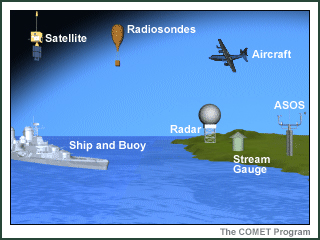
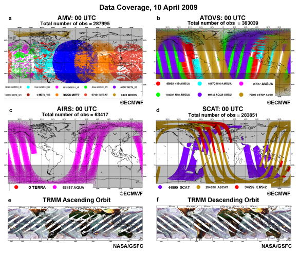
An additional challenge is the sparse network of surface and upper air observations in the tropics (Fig. 9.1). For vast regions of the tropics, such as the oceans and parts of Africa and the Americas, satellite sensors are the primary source of weather observations. While filling critical data gaps, satellite remote sensing has weaknesses that are described in Chapter 2. For example, polar-orbiting satellites view the same area at most twice per day and there are large gaps in the orbit paths across the tropics (Section 9.2.1.2).
An additional challenge is the sparse network of surface and upper air observations in the tropics (Fig. 9.1). For vast regions of the tropics, such as the oceans and parts of Africa and the Americas, satellite sensors are the primary source of weather observations. While filling critical data gaps, satellite remote sensing has weaknesses that are described in Chapter 2. For example, polar-orbiting satellites view the same area at most twice per day and there are large gaps in the orbit paths across the tropics (Section 9.2.1.2).
Numerical weather prediction (NWP) has been the key to rapid improvements in weather prediction in the midlatitudes but its benefits are yet to be fully exploited in the tropics. NWP presents its own challenges such as the need for parameterizations, difficulties with convective processes, and systematic errors1 related to the assimilation of sparse and heterogeneous data.
Tropical forecasters are faced with a variety of synoptic-scale systems that can produce heavy rain, strong winds, severe weather, dust storms, and high surf. The most hazardous of the synoptic systems are tropical cyclones (Chapter 8). Additional challenges such as blizzards can occur at high elevations in the Americas, Africa, and Asia. During the cool season, strong extratropical cyclones push cold fronts into the subtropics and tropics. While the temperature drop may be only a few degrees, cold fronts bring heavy rain, strong winds, and severe weather in prefrontal troughs or in the wake of the cold front. The monsoon regimes of the tropics generate monsoon depressions, monsoon gyres, and tropical cyclones. Even over relatively homogeneous tropical oceans, westerly wind bursts (Chapter 4) can produce gale-force winds. Within the large-scale pattern set up by the synoptic environment are mesoscale and convective-scale systems. Most tropical convection is organized into mesoscale systems but tropical convection occurs at a range of scales: isolated thunderstorms (1-10 km, hour), mesoscale convective systems (100-500 km, day), synoptic-scale superclusters (1000-4000 km, week), and the MJO (~10000 km, weeks to months).
Tropical forecasters are faced with a variety of synoptic-scale systems that can produce heavy rain, strong winds, severe weather, dust storms, and high surf. The most hazardous of the synoptic systems are tropical cyclones (Chapter 8). Additional challenges such as blizzards can occur at high elevations in the Americas, Africa, and Asia. During the cool season, strong extratropical cyclones push cold fronts into the subtropics and tropics. While the temperature drop may be only a few degrees, cold fronts bring heavy rain, strong winds, and severe weather in prefrontal troughs or in the wake of the cold front. The monsoon regimes of the tropics generate monsoon depressions, monsoon gyres, and tropical cyclones. Even over relatively homogeneous tropical oceans, westerly wind bursts (Chapter 4) can produce gale-force winds. Within the large-scale pattern set up by the synoptic environment are mesoscale and convective-scale systems. Most tropical convection is organized into mesoscale systems but tropical convection occurs at a range of scales: isolated thunderstorms (1-10 km, hour), mesoscale convective systems (100-500 km, day), synoptic-scale superclusters (1000-4000 km, week), and the MJO (~10000 km, weeks to months).
Tropical weather forecasting cannot rely on midlatitude synoptic weather models or even climatology to meet these forecasting challenges. While midlatitude cyclones have readily observed pressure signatures, locating the pressure signature of many tropical weather systems can be difficult. Here we explore analysis tools and forecast methods appropriate to the unique complexity of tropical weather systems.
9.2 Observations
9.2 Observations »
9.2.1 The Global Observation System
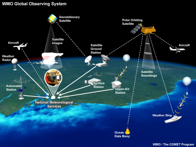
Observation is the first step in the process of weather analysis and prediction. Early weather observations were scattered and often depended on the interest and diligence of a single observer. The current global observing system has its origins in the observatories established in the 17th and 18th centuries, after the invention of the basic meteorological instruments (e.g., thermometer, barometer, hygrometer, and anemometer).2 The invention of the telegraph, in the 19th century, made it possible for observations to be transmitted in real-time. The formalization of international standards for practices, units, and observation types occurred at the International Meteorological Conference of Vienna in 1873.2 A global real-time surface network was in place by the early 20th century but the upper air network was not established until the 1940s. The satellite era of weather observations began in the 1960s with real-time coverage in the 1970s.
The present global observation system (Fig. 9.2) is comprised of instruments classified by the WMO3 as:
- Class 1 instruments, which measure in situ at a point; they occupy a small volume of the phenomena being measured (e.g., air temperature measured by ground station thermometer).
- Class 2 instruments, which measure area-averaged or volume-averaged variables remotely (e.g., temperature derived from satellite radiance or precipitation derived from radar reflectivity).
- Class 3 instruments, which measure wind velocity from tracking physical targets and their observed displacement with time (e.g., sondes tracked by Global Positioning Satellites or wind velocity derived from tracking cloud elements in satellite images).
The international meteorological observing system, overseen by the WMO, is the World Weather Watch (WWW). The WWW is comprised of the Global Observing System (GOS),4 the Global Telecommunication System (GTS), and the Global Data Processing System (GDPS). The systems are implemented and operated by the National Meteorological Services of WMO members. The rate of data collection and transmission is highly variable across the tropics. The situation is particularly dire in parts of Africa and the Americas. Many stations are no longer operational while others still collect data but cannot transmit that data because of telecommunication problems.5
WMO Global Telecommunication System, http://www.wmo.int/pages/prog/www/TEM/GTS/index_en.html
NOAA Observing Systems Architecture, http://www.nosa.noaa.gov/
Citizen Weather Observer Program, http://www.wxqa.com/
European Center for Medium-range Weather Forecast (ECMWF) data coverage maps,
http://www.ecmwf.int/products/forecasts/d/charts/monitoring/coverage/dcover
9.2 Observations »
9.2.1 The Global Observation System »
9.2.1.1 Point Observations
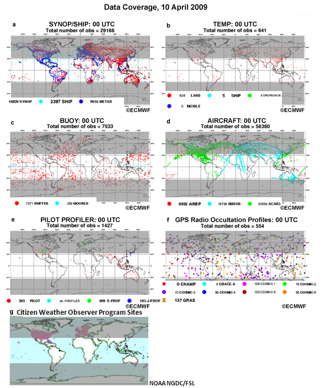
The WMO designated Regional Basic Synoptic Networks (RBSN) of surface and upper-air stations form the backbone of the station observation. Station observations are rare over the tropical oceans and sparse over parts of Africa and the Americas (Fig. 9.1). According to the WMO guidelines, surface synoptic stations should report every six hours (0000, 0600, 1200, 1800 UTC) for global exchange and every three hours within their regions. Each hour, routine aviation weather reports are sent and in between are special reports during extreme or rapidly changing weather. Supplemental surface weather data are contributed by citizen groups (Fig. 9.1g). Box 9-1 describes the standard weather elements observed and reported each hour.
The WMO designated Regional Basic Synoptic Networks (RBSN) of surface and upper-air stations form the backbone of the station observation. Station observations are rare over the tropical oceans and sparse over parts of Africa and the Americas (Fig. 9.1). According to the WMO guidelines, surface synoptic stations should report every six hours (0000, 0600, 1200, 1800 UTC) for global exchange and every three hours within their regions. Each hour, routine aviation weather reports are sent and in between are special reports during extreme or rapidly changing weather. Supplemental surface weather data are contributed by citizen groups (Fig. 9.1g). Box 9-1 describes the standard weather elements observed and reported each hour.
Upper-air stations are expected to report at least twice per day (usually 0000 and 1200 UTC) but many tropical stations only report once per day. Radiosonde wind measurements are calculated by following the instrument remotely and computing velocities from its displacement at fixed time intervals.
Station observations are the foundation of the global observation network but their sparseness in the tropics (Fig. 9.1) makes them inadequate for mesoscale analysis. Even for synoptic analysis, they must be supplemented with other observations. Appendix A describes how to plot surface and upper air observations on a weather map.
Station observations are the foundation of the global observation network but their sparseness in the tropics (Fig. 9.1) makes them inadequate for mesoscale analysis. Even for synoptic analysis, they must be supplemented with other observations. Appendix A describes how to plot surface and upper air observations on a weather map.
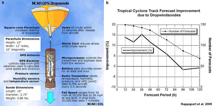
Instruments deployed for research field campaigns sometimes supplement routine weather observations and global data assimilation. For example, since 1997 the National Center for Atmospheric Research (NCAR) GPS Dropsonde system has provided high resolution vertical profiles of the atmosphere in support of operational weather forecasting and research. The first author was present when a dropsonde released from the NASA ER-2 aircraft during the 4th Convection and Moisture Experiment (CAMEX-4), provided the first stratosphere to surface profile of the eye of a tropical cyclone (Hurricane Erin 2001). The addition of dropwindsonde data has significantly improved tropical cyclone track forecasts—by 12-15% for the 12-48 h forecasts (Fig. 9.3).6
9.2 Observations »
9.2.1 The Global Observation System »
9.2.1.2 Remote Sensing: Area-averaged Observations
A simple overview of remote sensing observations is provided here; Chapter 2 has more details of remote sensing variables, applications, instruments, and platforms.
A simple overview of remote sensing observations is provided here; Chapter 2 has more details of remote sensing variables, applications, instruments, and platforms.
Satellite
Satellite remote sensing is the main source of routine tropical weather observations. Geostationary satellites plus polar and research satellites in low earth orbit (LEO) cover the global tropics (compare the coverage in Figs. 9.1 and 9.4), much of which is ocean.
Geostationary satellites offer wide spatial coverage and high temporal coverage (every 15-30 minutes) which makes them suitable for tracking weather phenomena, estimating winds from cloud driftestimating winds from cloud drift, nowcasting high impact weather, and data assimilation into NWP models. The next generation of geostationary satellites will have sensors currently available only on LEO, e.g., the geostationary lightning mapper on the GOES-R satellites will provide routine lightning observationslightning observations for weather analysis and forecasting.
LEO satellites offer high spatial resolution and are better suited for active instruments and microwave sensors. These satellites observe precipitation, winds, water vapor, lightning, and air quality. However, they have low temporal resolution and need a constellation to ensure a reasonable temporal sampling. Currently, significant gaps in coverage occur between LEO satellite swaths across the tropics (Fig. 9.4). The planned Joint Polar Satellite System (JPSS, formerly NPOESS) and Global Precipitation Measurement (GPM) mission, in combination with the European MetOp satellite, will dramatically improve coverage and the number of observations (Chapter 2, Focus 2Chapter 2, Focus 2).
Another critical tropical data void that satellites fill is atmospheric sounding. In addition to soundings from geostationary and LEOsoundings from geostationary and LEO satellites temperature and humidity profiles are derived from the occultation of signals from GPS satellitestemperature and humidity profiles are derived from the occultation of signals from GPS satellites. Real-time soundings from the Constellation Observing System for Meteorology, Ionosphere, and Climate (COSMIC) are available from http://www.cosmic.ucar.edu/.
Radar
Weather radar observations are very sparse in the tropics because ground-based radars are few and satellite-based radars, the Tropical Rainfall Measurement Mission (TRMM) Precipitation Radar and CloudSat, see each location at most twice per day. Individual radars are useful for analysis and forecasting over a small region. Far more useful is a network of radars coordinated as a mesoscale observation network to observe mesoscale circulations such as the core of tropical cyclones. Efforts are underway to create regional mosaics from adjacent radars in regions such as the Caribbean7 and Southeast Asia.8 For most of the tropics, precipitation is estimated from combinations of TRMM Precipitation Radar, geostationary IR, and LEO microwave observations (Chapter 2, Focus Section 2).
Weather radar observations are very sparse in the tropics because ground-based radars are few and satellite-based radars, the Tropical Rainfall Measurement Mission (TRMM) Precipitation Radar and CloudSat, see each location at most twice per day. Individual radars are useful for analysis and forecasting over a small region. Far more useful is a network of radars coordinated as a mesoscale observation network to observe mesoscale circulations such as the core of tropical cyclones. Efforts are underway to create regional mosaics from adjacent radars in regions such as the Caribbean7 and Southeast Asia.8 For most of the tropics, precipitation is estimated from combinations of TRMM Precipitation Radar, geostationary IR, and LEO microwave observations (Chapter 2, Focus Section 2).
9.2 Observations »
9.2.1 The Global Observation System »
Box 9-1 Weather Observations
The systematic gathering of basic meteorological elements is vital to the understanding of tropical weather systems, seasonal changes associated with these systems, and the variability of the tropical climate. The basic weather elements are: air pressure, air temperature, humidity, clouds, wind speed and direction, precipitation, and visibility. Many variables derived from these basic elements are now standard for weather analysis, e.g., the vorticity, a measure of fluid rotation, is derived from the wind velocity.
International guidelines for instruments calibration and error characteristics and methods of measurements are established by the WMO.3 Weather observations are encoded for transmission via the GTS using guidelines established by the WMO.9 The most common observations are surface hourly synoptic (SYNOP), hourly and special observations for aviation (METAR), radiosonde (TEMP) at 0000 and 1200 UTC. Observations from buoys (BUOY), ships (SHIP), and aircraft (AIREP) also contribute to the network. As new instruments and new products become available for weather analysis, new codes and transmission methods are developed through international cooperation and consensus. As mentioned in Section 9.2.1.1, operational forecasting benefits from observations created for research programs. For example, the TRMM satellite, intended to be a short-term research platform, became an integral part of tropical weather analysis. Data collected by NOAA and NASA research aircraft have been transmitted to NOAA operational centers in real-time. The Africa Monsoon Multidisciplinary Analysis (AMMA) added new instruments and resuscitated dormant stations over West Africa.5
During the past two decades, new satellite and marine instruments have dramatically improved tropical forecasts. The TAO-Triton, PIRATA, and RAMA buoy arrays provide critical observations over the tropical oceans. Assimilation of radiances from satellite instruments such as Advanced Microwave Sounding Unit (AMSU),10 Atmospheric Infrared Sounder (AIRS),11,12 Moderate Resolution Imaging Spectroradiometer (MODIS), and WindSAT13 has reduced forecast errors.
During the past two decades, new satellite and marine instruments have dramatically improved tropical forecasts. The TAO-Triton, PIRATA, and RAMA buoy arrays provide critical observations over the tropical oceans. Assimilation of radiances from satellite instruments such as Advanced Microwave Sounding Unit (AMSU),10 Atmospheric Infrared Sounder (AIRS),11,12 Moderate Resolution Imaging Spectroradiometer (MODIS), and WindSAT13 has reduced forecast errors.
9.2 Observations »
9.2.1 The Global Observation System »
9.2.1.3 Observation Error
Observations serve to characterize the state of the atmosphere as accurately as possible. The defining characteristics of an observation network are the variables being measured, the instrument errors, and the spatial and temporal distribution of measurements. Errors in observations can be caused by poorly calibrated instruments,14 instrument siting,14 and human observer error.15 Observation error can be categorized as:
- Instrument error, a function of instrument design and operating conditions. For example, dry bias in a commonly-used radiosonde was discovered during the TOGA-COARE experiment in the tropical West Pacific. The dry bias was about 2% up to the midtroposphere and 15% above 300 hPa.16 Similar bias was found for radiosonde measurements over West Africa17 during AMMA in 2006. Instrument bias18 is corrected by comparing with independent reference measurement. Relative humidity errors in the tropics are often the result of poorly ventilated instrument shelters. Excess solar radiation evaporates moisture during and after rain and causes an artificially high value of water vapor content.
- Error of representativeness, error caused by the misrepresentation of scales smaller than the distance between observation points. Since thunderstorms are on the order of 10 km, stations that are 100 km apart will miss thunderstorms between stations but will be adequate for observing synoptic-scale cyclones. For area-averaged measurements, weighted filters are used to remove small-scale variability and reduce the error. The surface wind velocity over land is strongly influenced by local-scale circulation and is not representative of the synoptic flow. However, the wind speed is still necessary for estimating evaporation (Chapter 5, Section 5.1.3)estimating evaporation (Chapter 5, Section 5.1.3).
- Observer error, such as the tendency of observers to favor particular values (e.g., values divisible by 5 or 10) or to under report small amounts of precipitation.15 Such errors are difficult to quantify and correct because the values appear reasonable. Solutions for reducing observer error include better training and more automated weather stations.
9.2 Observations »
9.2.1 The Global Observation System »
9.2.1.4 Status of Current and Future Observing Systems
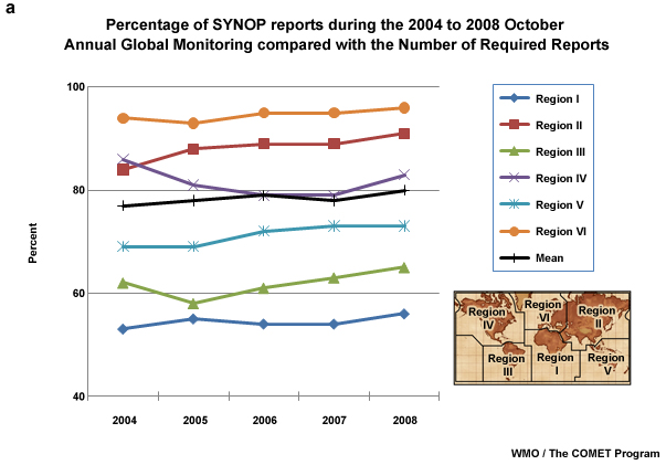
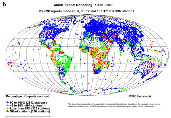
Current surface and upper air observing systems are monitored twice per year by the WMO World Weather Watch (WWW). In some regions, such as tropical Africa, the numbers of observations have decreased during recent decades. Figure 9.5 shows the trend and geographic distribution of how frequently stations are reporting observations. Most of the stations in the tropics have a less than 50% rate of reporting and many are “dead” stations (Fig. 9.5b). Efforts are underway to reverse that trend in some regions. For example, through the African Monsoon Multidisciplinary Analysis (AMMA) program, operational agencies in Africa and AMMA scientists have been reactivating silent stations, renovating others, and installing new stations in West Africa.5
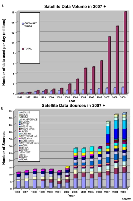
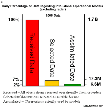
The increasing volume of satellite data (Fig. 9.6), while welcome, presents a challenge for operational forecast centers. Approximately 6 million elementary satellite observations are used for data assimilation into NWP models each day; a small fraction of satellite observations (Fig. 9.6c). However, the data are very inhomogeneous in quality and in spatial and temporal resolution. Nevertheless, forecasters need to understand how to exploit the new data for improvement in analysis and forecasting of tropical weather.
The increasing volume of satellite data (Fig. 9.6), while welcome, presents a challenge for operational forecast centers. Approximately 6 million elementary satellite observations are used for data assimilation into NWP models each day; a small fraction of satellite observations (Fig. 9.6c). However, the data are very inhomogeneous in quality and in spatial and temporal resolution. Nevertheless, forecasters need to understand how to exploit the new data for improvement in analysis and forecasting of tropical weather.
European Center for Medium-range Weather Forecast (ECMWF) data coverage maps,
http://www.ecmwf.int/products/forecasts/d/charts/monitoring/coverage/dcover
9.3 Weather Analysis
In order to forecast the weather, the forecaster needs to analyze the current weather. The primary tool of weather analysis is the weather map, on which all available data, needed to accurately depict the state of the atmosphere, are plotted. The scale of the weather phenomena being forecasted determines how frequent or dense the observations need to be. For example, short-term weather forecasts require very frequent observations over a small area while planetary-scale, long-range forecasts require a much less dense and less frequent network of observations. In recent decades, weather observation plotting has become an automated computer task but the manual method is still used in some tropical forecast centers.
Forecasters use a variety of analysis tools to examine phenomena in each scale starting with the global circulations such as the Intertropical Convergence Zone (ITCZ) and moving downscale to the intraseasonal Madden-Julian Oscillation (MJO) phase. Applying the concept of the forecast funnel, the next analysis scale is the synoptic weather, followed by the mesoscale, and finally, especially for nowcasting, the convective scale. Although we will identify common practices that should reduce wide variability, weather analysis is subjective. Even skilled analysts can create quite different analyses from similar observations.19
Forecasters use a variety of analysis tools to examine phenomena in each scale starting with the global circulations such as the Intertropical Convergence Zone (ITCZ) and moving downscale to the intraseasonal Madden-Julian Oscillation (MJO) phase. Applying the concept of the forecast funnel, the next analysis scale is the synoptic weather, followed by the mesoscale, and finally, especially for nowcasting, the convective scale. Although we will identify common practices that should reduce wide variability, weather analysis is subjective. Even skilled analysts can create quite different analyses from similar observations.19
In the next several subsections, we will examine a variety of tools commonly used for tropical weather analysis, from flow pattern analysis to remote sensing products, and finally, computer applications that help forecasters to synthesize observations and numerical model forecasts.
9.3 Weather Analysis »
9.3.1 Analysis Tools
9.3 Weather Analysis »
9.3.1 Analysis Tools »
9.3.1.1 Velocity Potential and Stream Function
In general, the tropical wind field provides more information about synoptic conditions than the pressure or geopotential height field. According to Helmholtz’s theorem, the wind velocity can be separated into two components:
 (1)
(1)The rotational wind,  , has all of the vorticity and no divergence and
  has all of the divergence and no vorticity. Vorticity, a measure of the local rotation of the flow, is calculated as the cross product of the vector windVorticity, a measure of the local rotation of the flow, is calculated as the cross product of the vector wind and has units of inverse seconds (s-1). Divergence measures the spreading out of the flow (also with units of s-1). Figure 9.7 illustrates the differences between the rotational and divergent components of the wind velocity. The two components can be further broken down into variables that are useful for tropical weather analysis, the stream function,
  , and velocity potential, χ:
 (2)
(2)Divergent wind,
 (3)
(3) Rotational winds are parallel to the stream function contours and their speeds are proportional to the stream function gradient. Divergent winds flow out low velocity potential and their speed is proportional to the gradient of velocity potential (Fig. 9.7b,c). Velocity potential and stream function are defined at the equator which makes them useful for model initialization in the tropics.
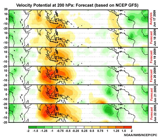
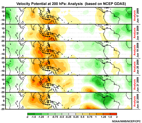
Because the velocity potential is proportional to divergence, it can be used to track regions of upper-level divergence where convection is enhanced (Fig. 9.8). Divergence from deep convection drives tropical circulations.
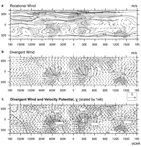
Anomalies or deviations from the mean velocity potential are much more useful than actual values for distinguishing the regions of deep convection or suppression. Figure 9.8 illustrates the correspondence between 200 hPa velocity potential anomalies and deep convection identified by enhanced satellite IR imagery. In this example, the ITCZ can be identified as the broken band of convection extending from Central Africa west to the central Pacific. A broad area of deep convection is apparent over the Western Pacific.
MJO indices, http://www.cpc.ncep.noaa.gov/products/precip/CWlink/MJO/index.primjo.html
Use of streamfunction and vorticity to objectively diagnose tropical waves,
http://www.atmos.albany.edu/student/gareth/diagnostics.html
NOAA/NWS Tropical Prediction Center Analysis Tools,
http://www.nhc.noaa.gov/analysis_tools.shtml
Tropical Analysis Charts, http://nomads.ncdc.noaa.gov/ncep/NCEP
9.3 Weather Analysis »
9.3.1 Analysis Tools »
9.3.1.2 Kinematic Analysis: Streamlines and Isotachs
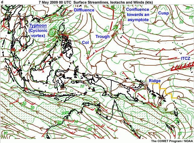
Kinematic analysis creates a continuous representation of the wind field from observations of the horizontal wind velocity. Although the stream function is a better variable than isobars for low latitude weather analysis, it is not the best representation of the air flow. Streamlines and isotachs provide more details of the horizontal flow at a given level than isobars (Fig. 9.9a, d, and e). Streamlines are lines that represent the flow tangential to the instantaneous wind direction. Forecasters use streamline analysis to identify many features. Figure 9.9d shows examples of the following features:
- Vortices – cyclonic or anticyclonic circulation centers and cyclonic and anticyclonic inflow and outflow. Streamlines form a closed curve around or emanate towards or away from that singular point. Low-level cyclonic inflow coincides with low pressure and anticyclonic outflows coincide with high pressure. At upper levels, anticyclonic outflow occurs above intense convective systems such as tropical cyclones. Upper level data is generally too sparse to determine the exact characteristics of inflow and outflow but in general cyclonic inflow and anticyclonic outflow are favored.
- Waves – perturbations in the streamlines that are similar to troughs and ridges in pressure or geopotential analysis.
- Asymptotes – streamlines of confluence, towards which nearby streamlines move; or diffluent asymptotes, from which nearby streamlines move away. Confluence (diffluence) may be associated with horizontal mass convergence (divergence) but that correlation is dependent on the distribution of the wind speed.
- Neutral points – points at which two asymptotes appear to intersect and the wind is calm. These points are also referred to as “cols”, or “saddles” between two areas of anticyclonic flow or two areas of cyclonic flow.
- Cusps – intermediate pattern between a wave and a vortex.
In Figure 9.9 (a,b), both the streamline analysis and the isobaric analysis identify the tropical cyclone over the South China Sea, the ridge across Australia, and a cyclone over the northeast Pacific. However, only the streamline analysis (Fig.9.9b) shows the South Pacific Convergence Zone, including the cyclonic circulations of the cloud clusters. Confluence into the ITCZ on the eastern edge of the domain is also evident in the streamline analysis.
The plots in Fig. 9.9 are generated by an automated analysis system. However, the methods used to create the plots can make mistakes because of lack of data or bad data points.
Can you identify a significant cyclonic feature that the automated analysis missed?
Feedback:
The automated analysis did not identify Tropical Storm Kujira (Fig. 9.10). However, the storm is present in the Unified Surface Analysis created by forecasters at the U.S. National Weather Service, Ocean Prediction Center, and Tropical Prediction Center. This example highlights the importance of the human forecasters, who synthesize all of the information and improve on the automated system, which in this case does not account for the satellite data.
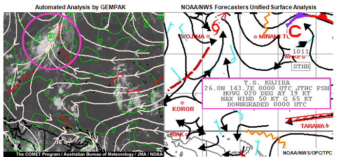
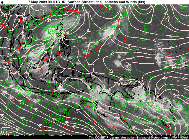
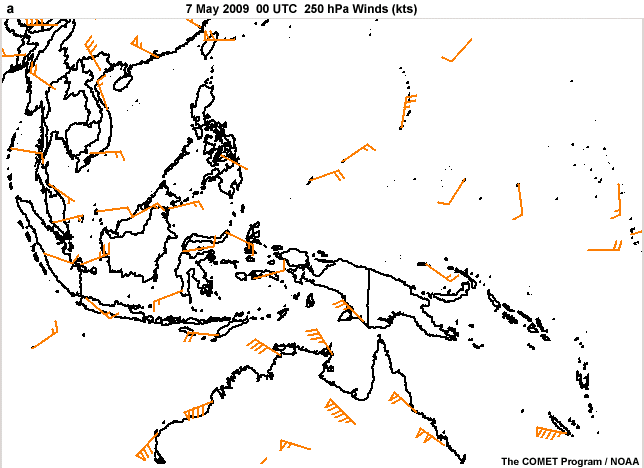
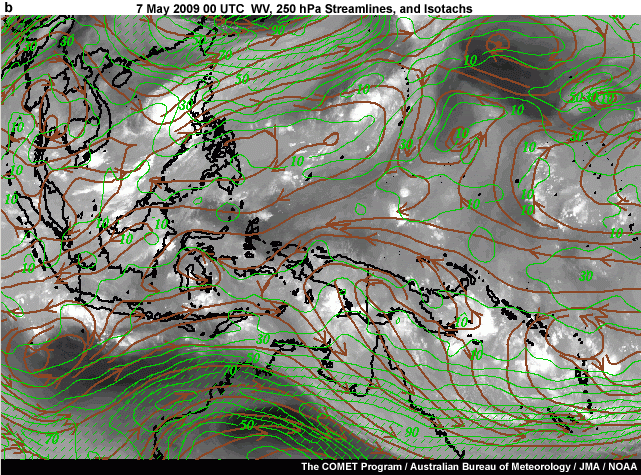
It is clear that the sparsely distributed station observations are insufficient to resolve all of the weather features, and therefore need to be supplemented by satellite products. Upper level streamline/isotach analysis is enhanced by the addition of satellite water vapor images (Fig. 9.11). The radiosonde observations resolve the jet stream speed and horizontal structure over Australia but do not fully resolve outflow from the two tropical cyclones.
9.3 Weather Analysis »
9.3.1 Analysis Tools »
9.3.1.3 Satellite Imagery
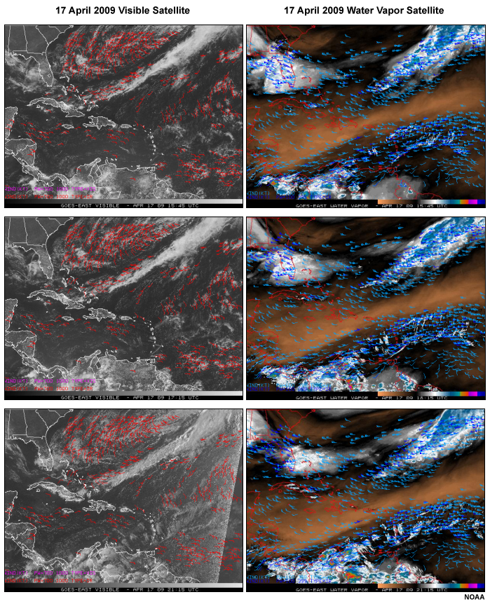
Satellite image analysis is an inherent part of tropical weather analysis because satellite coverage extends across the global tropics. As described in Chapter 2, various channels of the electromagnetic spectrum provide information about clouds, precipitation, winds, and air quality. For example, in Fig. 9.12 (left panels), visible images show clouds moving eastward from South America to the eastern Caribbean and Atlantic while other clouds are moving westward from the Atlantic to Central America. The water vapor imagery (right panels) confirms that air with high water vapor content in the upper troposphere is moving eastward. Animation of the IR images with color enhancement of cold cloud tops also allows us to distinguish different cloud layers and their movement.
Satellite image analysis is an inherent part of tropical weather analysis because satellite coverage extends across the global tropics. As described in Chapter 2, various channels of the electromagnetic spectrum provide information about clouds, precipitation, winds, and air quality. For example, in Fig. 9.12 (left panels), visible images show clouds moving eastward from South America to the eastern Caribbean and Atlantic while other clouds are moving westward from the Atlantic to Central America. The water vapor imagery (right panels) confirms that air with high water vapor content in the upper troposphere is moving eastward. Animation of the IR images with color enhancement of cold cloud tops also allows us to distinguish different cloud layers and their movement.
The sharp edge of the cold frontal clouds, extending northeast to southwest across the Atlantic, is evident in the visible images. The eastward flow at the upper levels is associated with the subtropical jet stream which has wind speeds greater than 40 m s-1; as derived from cloud motion vectors (Fig. 9.12, right). Wind velocity in the lower troposphere is derived from visible images of clouds (Fig. 9.12, left).
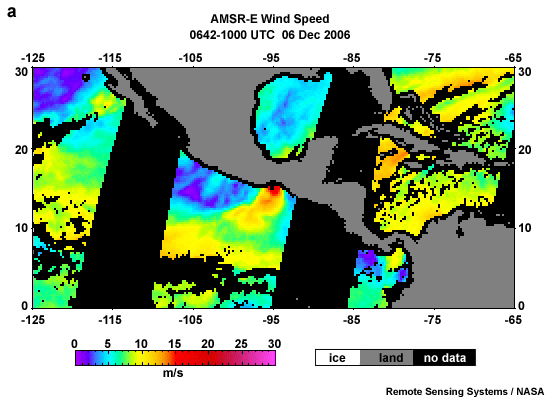
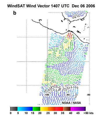
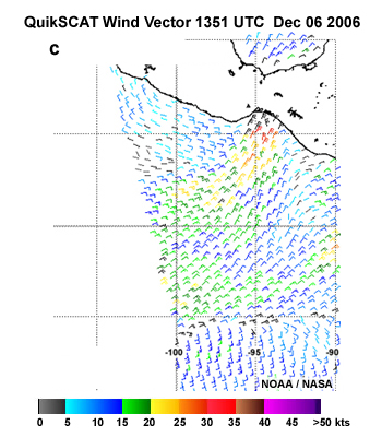
More precise surface winds are derived from LEO satellite microwave measurements. For example, Fig. 9.13, shows a low-level jet in the Gulf of Tehuantepec, a common phenomenon associated with "northers" or winter cyclones. As explained in Chapter 2, Section 2.7, scatterometry derives wind velocity by measuring backscatter from small-scale waves and foam. However, because wind retrievals can be ambiguous during rain, corrective factors have been created by data providers at NASA, NOAA, and EUMETSAT (both corrected and uncorrected wind fields are available).
More precise surface winds are derived from LEO satellite microwave measurements. For example, Fig. 9.13, shows a low-level jet in the Gulf of Tehuantepec, a common phenomenon associated with "northers" or winter cyclones. As explained in Chapter 2, Section 2.7, scatterometry derives wind velocity by measuring backscatter from small-scale waves and foam. However, because wind retrievals can be ambiguous during rain, corrective factors have been created by data providers at NASA, NOAA, and EUMETSAT (both corrected and uncorrected wind fields are available).
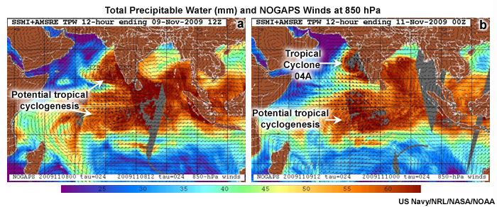
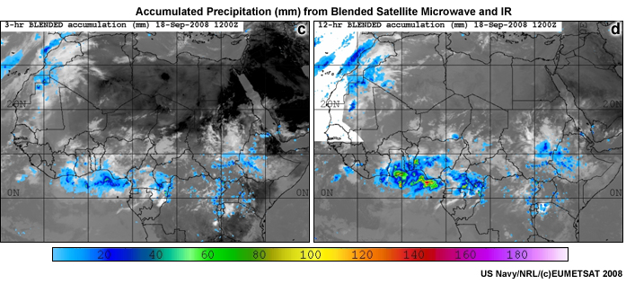
Moisture fields derived from satellite microwave measurements are especially critical for tracking synoptic features over the tropical oceans while combinations of LEO microwave and geostationary measurements provide precipitation estimates. The latter is especially critical because of the dearth of routine radar coverage. Figure 9.14a shows how satellite-derived total precipitable water (TPW) is combined with global model analysis to aid in forecasting tropical cyclogenesis in the Indian Ocean. Animations of TPW are useful for tracking the movement of tropical waves. Precipitation accumulations are estimated by blending measurements from TRMM Precipitation Radar, microwave, and geostationary IR (Fig. 9.14b).
Given the importance of satellite images to tropical weather analysis and forecasting, continuing education of tropical forecasters is necessary. Internet and other digital technologies are being exploited to enhance training in satellite interpretation for the tropics and elsewhere. For example, forecasters in the Caribbean, Central America, and South America have virtual monthly weather briefings, which use satellite images, animations, and allow participants to communicate using audio, text, and screen annotations.
http://rammb.cira.colostate.edu/training/rmtc/focusgroup.asp
WMO-CGMS Virtual Laboratory for Education and Training In Satellite Meteorology
http://www.wmo-sat.info/vlab/
Report on Centers of Excellence in Satellite Training,
http://www.wmo-sat.info/vlab/regional-focus-groups/
http://manati.orbit.nesdis.noaa.gov/cgi-bin/quikscat_amb_glo.pl
Real-time 3-hourly tropical rainfall analysis,
http://precip.gsfc.nasa.gov/rain_pages/3hrly.html
9.3 Weather Analysis »
9.3.1 Analysis Tools »
9.3.1.4 Radar Imagery
Operational weather radars in the US NWS scan in: (i) Clear Air Mode that is, typically, more sensitive, detects bugs, dust and is useful for identifying boundaries such as gust fronts; (ii) Precipitation Mode that detects precipitation and storm structure but is less sensitive.
Reflectivity
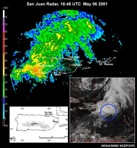
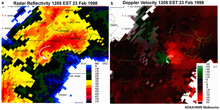
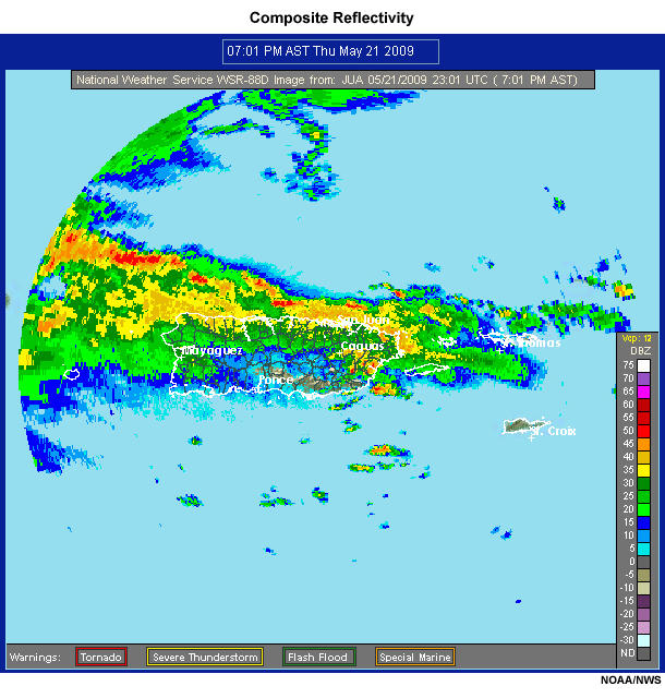
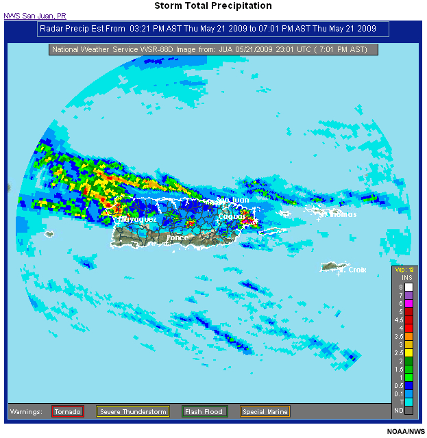
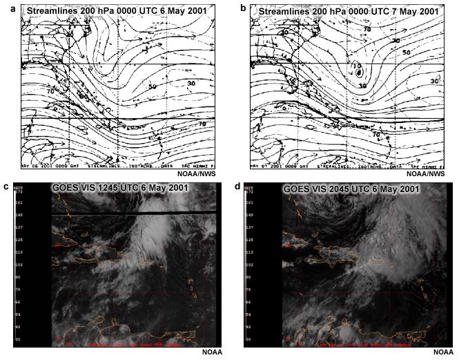
The most frequently used radar images are base and composite reflectivity, which show the location, intensity, and type of precipitation (e.g., Fig. 9.15). The Plan Position Indicator (PPI) radar display is used to analyze the horizontal structure of convective weather systems. Radar observations help refine the placement of frontal boundaries and gust fronts. The latter is often only evident when radars scan in clear air mode. Animations of radar images are valuable for short-term forecasting or nowcasting of severe weather and flash floods. For example, on 6 May 2001, areas in western Puerto Rico experienced flash floods that killed two people and caused damage worth $146 million.20 While the visible satellite image, in Fig. 9.15, shows widespread cloudiness associated with the trough, the radar reflectivity image shows the detailed structure of the precipitation. Within the large precipitation band are several heavy precipitation cells, with the heaviest concentrated over the southwestern part of the island. Animation of the radar image shows hours of heavy precipitation over that region where convection was enhanced by orographic uplift along the “Cordillera Central” (inset map, Fig. 9.15).
The PPI reflectivity scans capture the distribution of convective and stratiform precipitation in a tropical squall line passing over Niger, West Africa (Fig. 9.16a). The propagation velocity of various features, such as the convective line or the gust front, can be estimated.
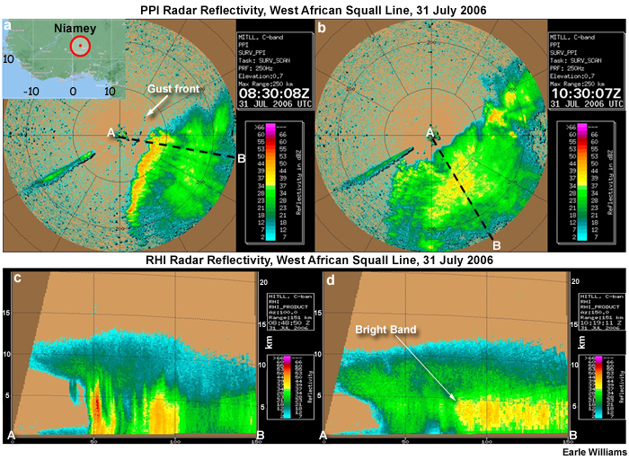
Vertical scan or Range Height Indicator (RHI) display is another useful tool for analysis and forecasting. The RHI images show strong reflectivity in the convective updrafts, up to 13 km (Fig. 9.16b). The convective downdrafts and updrafts, at the leading edge of the squall line, are of special interest to aviation forecasters who issue severe turbulence warnings. Later in the lifecycle of the squall line, the convective line decays but stratiform precipitation continues. The bright band of strong reflectivity just below 5 km is associated with melting ice particles.
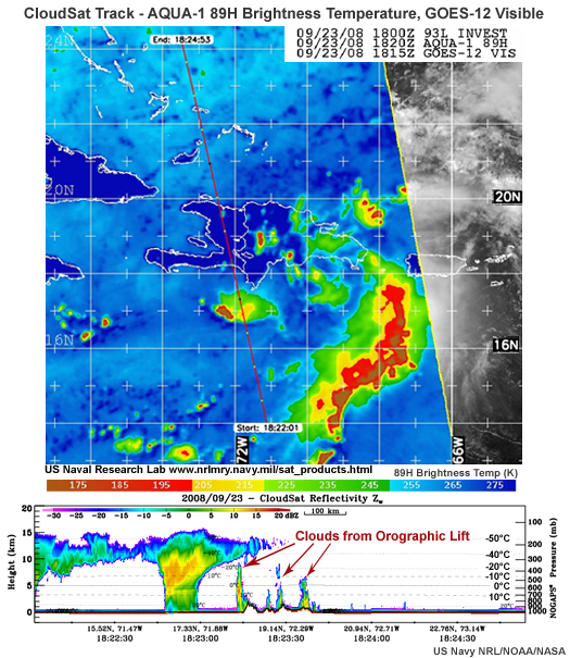
Radars can also be used to estimate cloud geometry. CloudSat, a satellite-based cloud radar primarily focused on climate studies, can also be used to analyze the vertical structure of clouds where orbits are favorable (e.g., Fig. 9.17). In places without ground-based weather radar, the TRMM PR and CloudSat provide the only information about the vertical structure of storms. See Chapter 2, Focus Section 2 for more information about the TRMM PR and CloudSat.
Radars can also be used to estimate cloud geometry. CloudSat, a satellite-based cloud radar primarily focused on climate studies, can also be used to analyze the vertical structure of clouds where orbits are favorable (e.g., Fig. 9.17). In places without ground-based weather radar, the TRMM PR and CloudSat provide the only information about the vertical structure of storms. See Chapter 2, Focus Section 2 for more information about the TRMM PR and CloudSat.
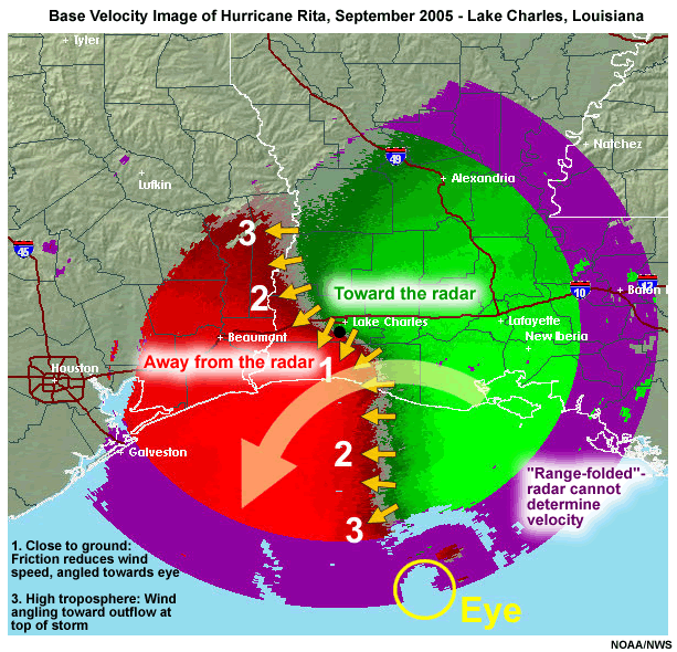
Forecasters can glean more information about mesoscale and convective scale phenomena from Doppler radar wind velocity images. Using the case of Hurricane Rita near landfall, we can understand how to interpret velocity images (Fig. 9.18). The green areas indicate movement toward the radar and red areas indicate movement away from the radar. The yellow arrows show the general counter-clockwise motion around the eye. Remember that the radar beam is angled upward which means that farther observations are at higher altitude. For instance, in the image of Rita, numbers 1 to 3 indicate winds at increasing distance and altitude.
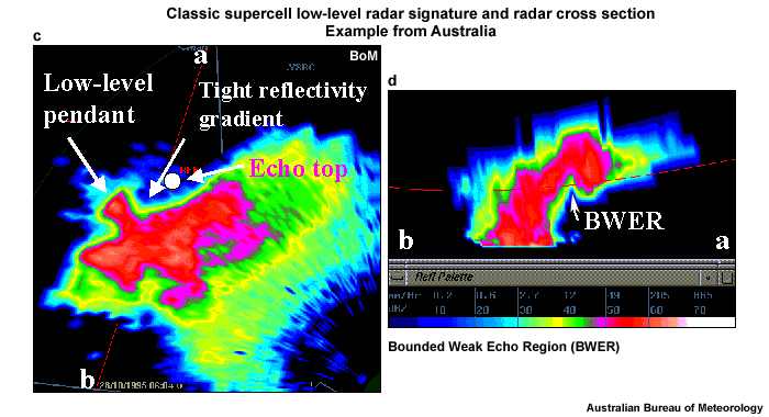
Doppler velocity is very useful for the identification of mesocyclones and tornadoes (Fig. 9.19). The signature is a velocity couplet indicating the mesocyclone circulation (indicated by the white arrow in Fig. 9.19b). The reflectivity signature is referred to as a “hook” echo because of its shape (white arrow in Fig. 9.19a). Fig. 9.19c is an example of a hook echo observed over Australia. In the cross-section of Figure 9.19d, the weak echo region bounded by high reflectivity indicates a strong updraft.
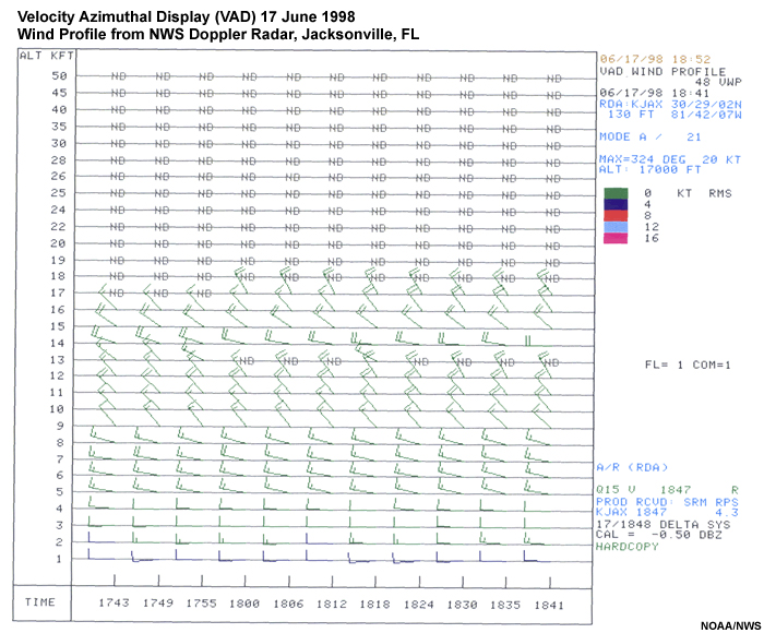
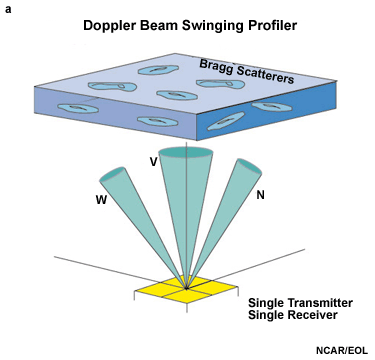
The Doppler velocity can also be used to derive an averaged wind profile. A Velocity Azimuth Display (VAD) wind profile is a time-height display of wind velocity (Fig. 9.20). It is derived from a volumetric sample of backscatter from dust, insects, and cloud droplets. The VAD wind profile is used to diagnose vertical wind shear, the depth of the boundary layer, and boundaries such as fronts, dry lines or sea breezes.
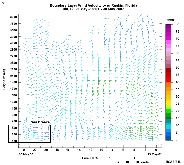
Time-height plots of velocity are also obtained from wind profilers, which operate on the same principle as Doppler radar except that they point vertically from the surface. For example, Fig 2.12b shows wind profiler observations of the sea breeze over west Florida.
Time-height plots of velocity are also obtained from wind profilers, which operate on the same principle as Doppler radar except that they point vertically from the surface. For example, Fig 2.12b shows wind profiler observations of the sea breeze over west Florida.
Precipitation
On a daily basis, a large community of users is interested in knowing when, where, how much, and what type of precipitation to expect. For example, quantitative precipitation estimates and forecasts are needed to manage agriculture, water resources, and renewable energy. Radar data provide high resolution spatial and temporal information on rainfall (Fig. 9.21) distribution which is useful for forecasting normal precipitation as well as high impact hydrometeorological events such as flash floods.
Precipitation is derived from relating a reflectivity factor, Z, to the number and size of raindrops per cubic meter (a measure of rainfall rate, R).
where Z is the reflectivity factor, D is the drop diameter, and N(D) is the number of drops of given diameter per cubic meter. “Z-R” relationships make assumptions about the drop size distribution of hydrometeors encountered by the radar beam. Different Z-R relationships are used for different atmospheric conditions. For example, a “convective” Z-R relationship is used with warm moist air and high concentrations of large droplets. Errors in radar-derived precipitation result from:
- variations in drop-size distributions (a small number of large hydrometeors can have the same reflectivity value as a very large number of smaller drops)
- the phase of precipitation (melting snowflakes can be identified as large raindrops which leads to an overestimate of rainfall rate)
- lack of low-level information
Polarimetric radar can improve the accuracy of precipitation when compared to standard Z-R methods because they differentiate between echoes from hydrometeors and non-hydrometeors and improve classification of hydrometeor types.21,22 Learn more about radar precipitation estimates in COMET Module, Precipitation Estimates, Part I: Measurement, http://www.meted.ucar.edu/hydro/precip_est/part1_measurement/
Radar observations are least useful in complex terrain or heavily urbanized areas, where the radar beam can be blocked. You may review the basics of weather radar in Chapter 2, Section 2.2 and link to online tropical radar images from Chapter 2, Appendix A.
Radar observations are least useful in complex terrain or heavily urbanized areas, where the radar beam can be blocked. You may review the basics of weather radar in Chapter 2, Section 2.2 and link to online tropical radar images from Chapter 2, Appendix A.
http://www.srh.noaa.gov/srh/jetstream/doppler/doppler_intro.htm
Dual Polarization Radar Training,
http://www.wdtb.noaa.gov/modules/dualpol/
9.3 Weather Analysis »
9.3.1 Analysis Tools »
9.3.1.5 Thermodynamic Diagram: Radiosonde Analysis
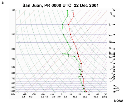
Radiosondes are released at 0000 and 1200 UTC each day and provide a vertical profile or "sounding" of the atmosphere. Vertical profiles are also provided by aircraft and satellite measurements. Thermodynamic diagrams (e.g., Skew-Temperature-LogPressure diagram, Fig. 9.22) help forecasters to determine the relative humidity, stability, vertical wind shear, severe weather, and flash flood potential of the atmosphere in the vicinity of the sounding. For instance, the sounding in Fig. 9.22a shows a deep layer of saturated and near saturated air up to 500 hPa, unstable temperature profile, weak mid-level shear, all of indicators of heavy rainfall. Additional factors in enhanced upward motion are strong mid-upper level shear associated with an upper-level trough and divergence; warm, moist easterly flow towards high terrain enhances orographic precipitation. Not surprising, this profile, with deep layer of moisture, near moist adiabatic temperature in the lower troposphere, and vertical wind shear to sustain long-lived convection and heavy precipitation, was associated flash floods in Puerto Rico.
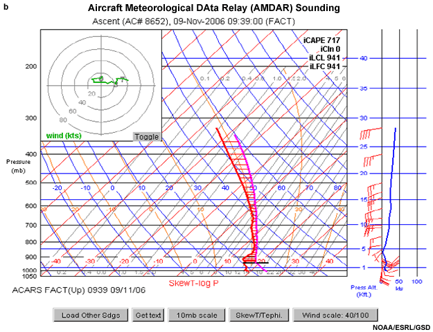
The AMDAR sounding (Fig. 9.22b) includes a hodograph plot on the upper left. The hodograph depicts the environmental vertical wind shear. The shear helps to determine storm type, structure, and evolution. Hodographs show the endpoints of wind vectors from the lowest to the highest level relative to a central point. The loop to the left in the hodograph (Fig. 9.22b) corresponds to the wind velocity change between the surface and 900 hPa. The hodograph and wind barb plots show strong directional shear at low-levels and increasing unidirectional wind shear in the upper levels. The area between the parcel and environmental temperature curve is the convective available potential energy (CAPE) (Chapter 5, Section 5.2.2.2), an indicator of instability.
The AMDAR sounding (Fig. 9.22b) includes a hodograph plot on the upper left. The hodograph depicts the environmental vertical wind shear. The shear helps to determine storm type, structure, and evolution. Hodographs show the endpoints of wind vectors from the lowest to the highest level relative to a central point. The loop to the left in the hodograph (Fig. 9.22b) corresponds to the wind velocity change between the surface and 900 hPa. The hodograph and wind barb plots show strong directional shear at low-levels and increasing unidirectional wind shear in the upper levels. The area between the parcel and environmental temperature curve is the convective available potential energy (CAPE) (Chapter 5, Section 5.2.2.2), an indicator of instability.
The representativeness of a sounding for the surrounding environment and for specific weather events are critical issues for forecasters. How do they adjust the “typical” sounding profile of, say, a hail producing thunderstorm, for their area? Review COMET Module, Skew-T Mastery, http://www.meted.ucar.edu/mesoprim/skewt/, for the basics of radiosonde analysis, critical parameters, and forecast applications.
Most forecast centers have programs to calculate and display key forecast parameters from thermodynamic diagrams. Critical information from the thermodynamic profiles includes:
- Stability – Is the troposphere stable or unstable? Where are the stable or unstable layers?
- Temperature – How close is the environmental temperature profile to the moist or dry adiabatic profile?
- Dewpoint – How close is it to the temperature profile? Where are the dry or moist layers?
- Lifting Condensation Level (LCL) – How high?
- Level of Free Convection (LFC) – How high?
- CAPE and Convective Inhibition (CIN) – Need to know amounts and vertical distribution of these measures of stability; they are proportional to the maximum updraft and downdraft speeds, respectively.
- Key indices such as:
- Lifted Index – Measures stability as the difference between the parcel and environmental temperature at 500 hPa; greater difference, more unstable.
- K index – High values indicate instability and heavy rainfall potential
- Total Totals Index – increasing values correspond to increasing potential for thunderstorms
- Precipitable Water Content – High values are associated with heavy precipitation and high precipitation efficiency
- Wind velocity – How strong? What is the vertical wind shear in the low, mid, upper troposphere?
- Hodograph - Indicates the vertical shear, which helps to determine the mode of convection.
- Storm Relative Environmental Helicity – an indicator of the potential for thunderstorms with rotating updrafts, i.e., the formation of supercells and tornadoes. It is sensitive to assumptions about storm motion and wind shear and is least useful with rapidly evolving environments.
9.3 Weather Analysis »
9.3.1 Analysis Tools »
9.3.1.6 Vertical Cross Sections
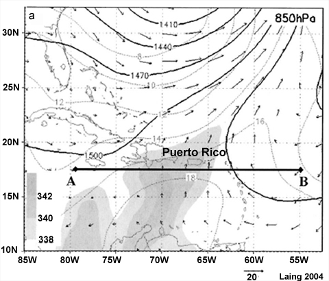
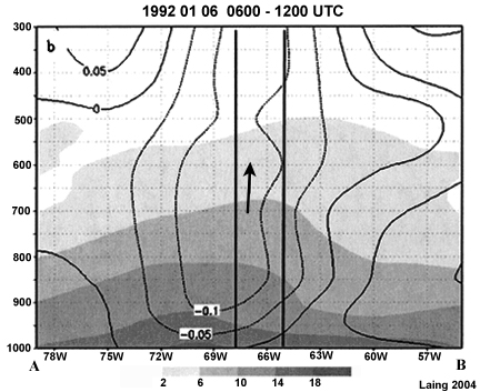
Upper air data, usually from radiosondes, provides information about the vertical structure of weather systems. Cross-sections through various layers provide information about where the air is rising or sinking, moist and dry layers, and the vertical extent of surface or upper tropospheric fronts. Using the Puerto Rico floods of 6 January 1992 as an example, we see an influx of air with high equivalent potential temperature (θe) at 850 hPa, one indicator of high flood potential (Fig. 9.23). A cross-section through the layer of high θe air reveals other ingredients for the deep convection and heavy rainfall over Puerto Rico: A deep layer of high specific humidity and rising motion.
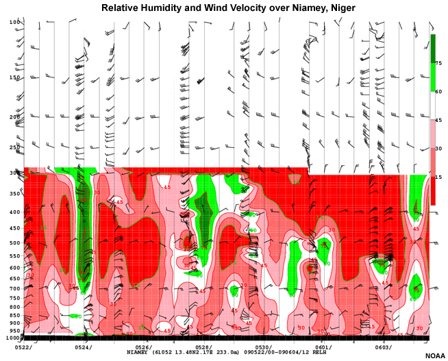
Time-height plots can be used to track synoptic-scale features such as African Easterly waves (Chapter 8). From the wind barbs and relative humidity we can identify several easterly waves moving across West Africa (Fig. 9.24). Waves have high relative humidity (green) and the wave trough is marked by winds in the low-mid troposphere shifting from northeasterly to southeasterly or southerly, e.g., on 24 May.
Time-height plots can be used to track synoptic-scale features such as African Easterly waves (Chapter 8). From the wind barbs and relative humidity we can identify several easterly waves moving across West Africa (Fig. 9.24). Waves have high relative humidity (green) and the wave trough is marked by winds in the low-mid troposphere shifting from northeasterly to southeasterly or southerly, e.g., on 24 May.
9.3 Weather Analysis »
9.3.1 Analysis Tools »
9.3.1.7 Trajectories
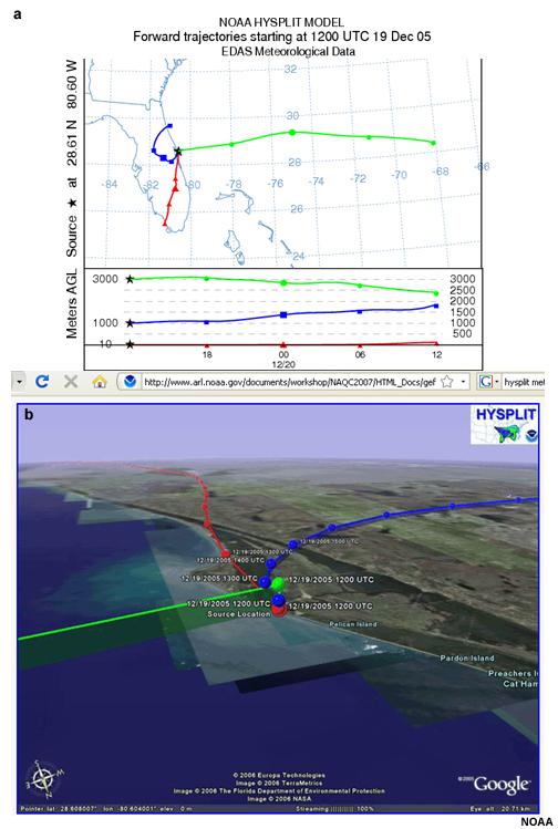
Trajectory analysis is used to monitor and forecast dispersion and deposition of pollutants such as volcanic ash, dust, smoke, and other aerosols. Air parcel trajectories are calculated by integrating data from discrete points in space and time (x,y,z,t) into a continuous function. Air pollution dispersal models have been adapted for various applications and regions. Most dispersion models ingest gridded NWP model output to calculate transport and diffusion of pollutant plumes. Backward trajectories are useful for determining the source region of pollutants in the forecast region of interest. Forward trajectories show where pollutants from a source region will travel.
The HYbrid Single-Particle Lagrangian Integrated Trajectory (HYSPLIT) is run by US National Weather Service, the Australian Bureau of Meteorology, and the Volcanic Ash Advisory Centers (VAAC). HYSPLIT trajectory maps typically show plan and vertical views of the air parcels paths (Fig 9.25); these can also be projected onto Google Earth (Fig. 9.25b). The position of the air parcel for a user-defined period is marked along the trajectory. HYSPLIT applies to gases and particles that have limited chemical reactivity and with neutrally buoyant releases. Like other dispersion models, HYSPLIT inherits errors from the underlying NWP model. HYSPLIT also has problems with flow and dispersion through complex terrain on scales not resolved by the meteorological model (HYSPLIT Applications for Emergency Decision Support, http://www.meted.ucar.edu/training_module.php?id=773).
NOAA Smoke Forecasts, http://www.arl.noaa.gov/smoke.php
Ocean Prediction Center, Volcanic Ash, http://www.opc.ncep.noaa.gov/volcano/
9.3 Weather Analysis »
9.3.1 Analysis Tools »
9.3.1.8 Marine Analysis
Marine forecasters predict the state of the ocean and other open waters such as large lakes. Of primary concern are waves: their steepness, height, velocity, period or wavelength, shoaling (where long waves become steep in shallow water), and degree of confusion (when different waves are present). For marine forecasts, we need to analyze:
- Winds
Wind stress is the primary driver of waves, so accurate marine wi0nd analysis and forecast are critical to marine forecasts. The wind stress, τ, varies as the square of the wind, τ = ρa CD U2, where ρa is the density of air, CD is the drag coefficient, (a measure of the roughness of the ocean surface determined empirically), U is the wind speed. Swells are waves that have moved out of its wind generation source region and are usually less steep than the original wave.
- Wave Speed and Wavelength
Wave speed depends on wavelength. For deep water waves, the longer the wavelength, the faster the wave speeds. Wave speeds slow as water becomes shallower and the waves become steeper. Note that wave group velocity (not individual wave speed) must be used to estimate the time it takes for waves/swell to arrive at a given location.
- Wave Height and Wave Energy
As wave height doubles, wave energy quadruples. This relationship is very significant in forecasting wave height. Forecasts of wave heights must be kept within a narrow range as inaccuracies in height are multiplied dramatically for wave energy and the potential for destruction.
Forecasters focus on forecasting "significant wave height" or “combined seas” and "peak wave period" while bearing in mind that a spectrum of waves make up the total sea state. Trained observers report wave heights that most often correlate with the mean height of the highest one third of the waves passing a point. Another useful operational concept is “Maximum Combined Seas”, the maximum height likely to occur when one or more wave groups pass a location simultaneously. The Maximum Combined Seas can be much greater than the height of any individual wave or swell, especially if there are multiple swells and/or wave groups with similar periods. Such situations can create waves with dramatic heights, so called rogue waves.
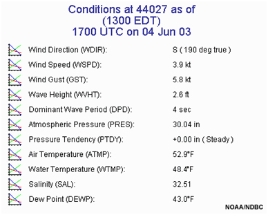
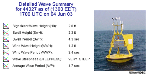
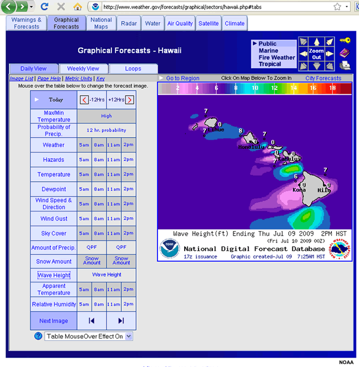
Observations of the sea state are obtained from buoys (Fig. 9.26) and from satellite sensors (Fig. 9.13a, 9.13b, 9.13c). The current network of ocean observations is shown in Figs. 9.1c and 9.4d. Observations are analyzed and combined with guidance from wave models to produce forecasts such as wave heights (Fig. 9.27).
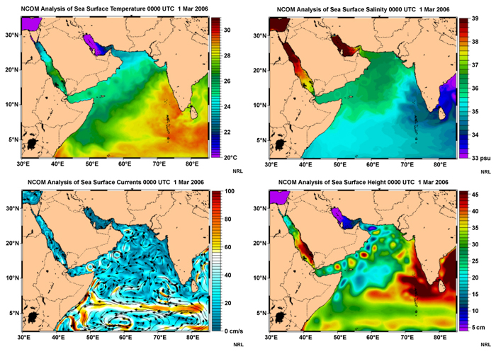
- Temperature, Salinity and Currents
Observations over the ocean suffer from sparseness and measurement errors. Ocean circulation models combine these observations with physics to create analyses for diagnosing temperature, salinity, currents, and sea height (Fig. 9.28).
A set of interactive wind and wave forecasting tools are available from COMET at http://www.meted.ucar.edu/marine/widgets/. You can learn more about wind and wave forecasting in the COMET distance learning course on wind and wave forecasting at http://www.meted.ucar.edu/dl_courses/Wind_Wave_Fcsting/.
NCEP Marine Forecasts,
http://mag.ncep.noaa.gov/NCOMAGWEB/appcontroller
NOAA/NWS/NCEP Ocean Prediction Center, http://www.opc.ncep.noaa.gov/
9.3 Weather Analysis »
9.3.1 Analysis Tools »
9.3.1.9 Synthesis
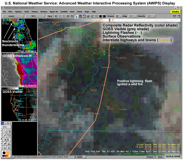
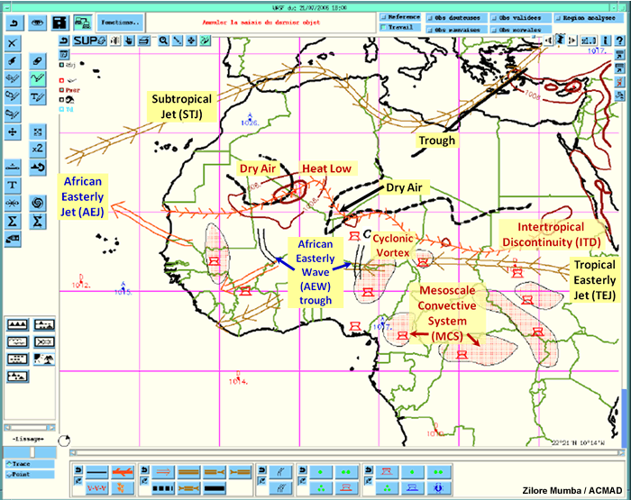
Modern digital tools allow forecasters to overlay a variety of data and zoom to assess the weather at various scales. In the following sections, we explore each scale in turn. Even in the modern era, manual skills are still useful to synthesize the information and to make adjustments where the automated techniques fail to capture critical features. Figure 9.29 shows two examples of operational display and analysis systems. The first one shows the overlay of radar, satellite, surface observations, and lightning flashes on a map of towns and highways. The radar reflectivity allows the forecaster to see the intensity and structure of the thunderstorm cells. The widespread cloudiness is shown by the grayscale visible satellite image. Station plots (peach) and lightning (green) show weather at specific locations. In the second example, from Synergie, colored symbols illustrate circulation features, weather systems, and boundaries to provide a synthesized picture of the weather.
NOAA/NWS Aviation Weather Analysis, http://aviationweather.gov/
Examples of synthesized tropical weather analysis
African Centre of Meteorological Application for Development (ACMAD),http://www.acmad.ne/en/homepage.htm
Unified Surface Analysis, http://www.opc.ncep.noaa.gov/Loops/#Unified_Surface_Analysis_Products
Tropical Analysis Charts, http://nomads.ncdc.noaa.gov/ncep/NCEP (choose from list)
South African Weather Service, http://www.weathersa.co.za/
NCEP International Desk Non-operational Products (may not be current or available on a routine basis)
http://www.hpc.ncep.noaa.gov/international/intl2.shtml#charts
http://www.hpc.ncep.noaa.gov/discussions/fxca20.html
http://www.hpc.ncep.noaa.gov/discussions/fxsa20.html
http://www.hpc.ncep.noaa.gov/international/scs/Columbia4.html
9.3 Weather Analysis »
9.3.2 Global-scale Circulations:Top of the Forecast Funnel
Now that we have identified various analysis tools, we are ready to start tropical weather analysis. Using the principle of the forecast funnel(from the large-scale to the small-scale), forecasters should be first aware of the climatology and the planetary circulations that affect their region.
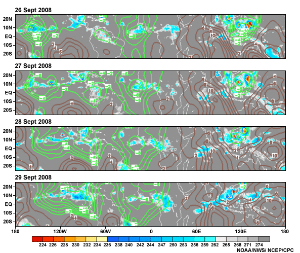
One of the most important features of the tropical atmosphere is the equatorial trough, the region of minimum surface pressure. The northeast and southeast trade winds converge into this low pressure, hence its other name, the InterTropical Convergence Zone (ITCZ). The ITCZ is usually identified as a belt of thunderstorms around the global tropics but it is not continuous and the cloud systems within it change every day (for example, see Fig. 9.8). The equatorial trough, convergence zones, and other surface circulations migrate through the year in response to surface heating (Fig. 9.30).
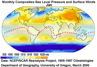
As illustrated in Fig. 9.30 (bottom panel), the trade winds converge north of the equator over the eastern Pacific. The convergence zone is known there as the Near Equatorial Trade Wind Convergence (NETWC). For Asia and Australia, the maximum heating and low pressure are in continental regions far from the equator. There the trough is part of the monsoon system and referred to as the Monsoon Trough. Flow into the monsoon trough is predominantly westerly (in contrast to easterlies elsewhere in the tropics). Flanking the equatorial trough are the subtropical highs and ridges, regions of subsidence.
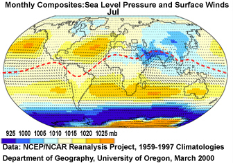
Two quasi-permanent and extensive convergence zones lead to tropical-temperate interactions: the South Pacific Convergence Zone (SPCZ)24 and the South Atlantic Convergence Zone (SACZ).25,26,27,28 The SPCZ and SACZ are oriented northwest to southeast from the tropics to the subtropics. They are broad features with precipitation extending more than 30° longitude (Fig. 9.31).
Forecasters should also be aware of the phase of ENSO and the typical climate impacts for their region. While the direct impacts are felt in the regions surrounding the tropical Pacific, ENSO affects many regions around the world. Real-time ENSO observations and forecasts sources are listed in Table 4.3.
Forecasters should also be aware of the phase of ENSO and the typical climate impacts for their region. While the direct impacts are felt in the regions surrounding the tropical Pacific, ENSO affects many regions around the world. Real-time ENSO observations and forecasts sources are listed in Table 4.3.
9.3 Weather Analysis »
9.3.3 Intra-seasonal Analysis for Tropical Weather Forecasting
The Madden-Julian Oscillation (MJO),29,30 the leading mode of tropical intraseasonal variability, produces extensive periods of enhanced or suppressed precipitation and modulates tropical cyclone activity (Chapter 4, Section 4.1.1.3). Therefore, tropical weather forecasters need to monitor the MJO. Currently, operational centers, such as the Australian BOM and the US NWS Climate Prediction Center (CPC),31 provide official weekly assessments and forecasts of the MJO (Fig. 9.32 and Chapter 4, Table 4.1). The CPC's prediction skill of an MJO Index (Chapter 4, Section 4.1.1.4) out to 7-10 days is modest but continues to improve. These forecasts are for existing MJO events as operational global models cannot presently predict the onset of an MJO.32
The Madden-Julian Oscillation (MJO),29,30 the leading mode of tropical intraseasonal variability, produces extensive periods of enhanced or suppressed precipitation and modulates tropical cyclone activity (Chapter 4, Section 4.1.1.3). Therefore, tropical weather forecasters need to monitor the MJO. Currently, operational centers, such as the Australian BOM and the US NWS Climate Prediction Center (CPC),31 provide official weekly assessments and forecasts of the MJO (Fig. 9.32 and Chapter 4, Table 4.1). The CPC's prediction skill of an MJO Index (Chapter 4, Section 4.1.1.4) out to 7-10 days is modest but continues to improve. These forecasts are for existing MJO events as operational global models cannot presently predict the onset of an MJO.32
The relationship of MJO phase and tropical cyclone genesis is valuable for tropical forecasting. MJO indices used as predictors of the probability of tropical cyclone formation increased forecast skill out to about three weeks for the south Indian and Pacific Ocean basins.33
Equatorial Waves
Intraseasonal equatorial waves also affect weather (Chapter 4, Focus 1), e.g., tropical cyclones form from equatorial Rossby and Mixed Rossby-gravity waves (MRG). Also daily rainfall is enhanced during the wet phase of eastward-moving Kelvin waves and suppressed during the dry phase. While most equatorial waves are identified by filtering of outgoing longwave radiation (OLR) and wind anomalies at 850 and 200 hPa (Chapter 4, Section 4.1.5.2) some can be identified from standard 850 and 200 hPa synoptic analysis.
Intraseasonal equatorial waves also affect weather (Chapter 4, Focus 1), e.g., tropical cyclones form from equatorial Rossby and Mixed Rossby-gravity waves (MRG). Also daily rainfall is enhanced during the wet phase of eastward-moving Kelvin waves and suppressed during the dry phase. While most equatorial waves are identified by filtering of outgoing longwave radiation (OLR) and wind anomalies at 850 and 200 hPa (Chapter 4, Section 4.1.5.2) some can be identified from standard 850 and 200 hPa synoptic analysis.
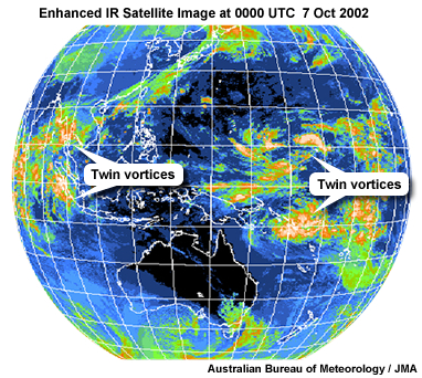
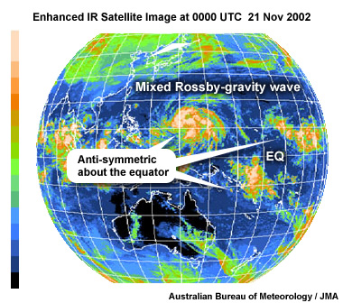
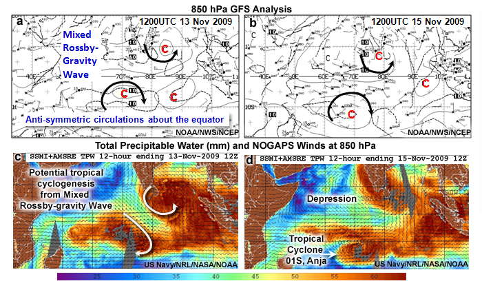
Equatorial Rossby waves are identifiable as cyclonic vortex twins in the Northern and Southern Hemispheres at 850 hPa (e.g., Fig. 9.33, Fig. 5.17, Fig. 8.21). Equatorial waves sometimes form in succession, e.g., in Fig. 9.33e,f. The large-scale pattern can also transition from Mixed Rossby to equatorial Rossby wave (Fig. 9.33a,b) and vice versa within a couple of days.
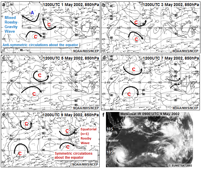
MRG waves are evident as anti-symmetric circulations about the equator, an anticyclonic circulation in one hemisphere and a cyclonic circulation in the opposite hemisphere (e.g., Fig. 9.33a, 9.34, Fig. 5.18, Fig. 8.22). Strong cross-equatorial flow between the high and the low at 850 hPa is another marker of MRG waves (Fig. 9.34c).
Analysis and forecast of equatorial waves are available in real-time from NOAA and the Australian BOM. The forecast skill for equatorial waves extends to half the lifetime of the waves, 1-5 days, depending on the type of wave.34
Analysis and forecast of equatorial waves are available in real-time from NOAA and the Australian BOM. The forecast skill for equatorial waves extends to half the lifetime of the waves, 1-5 days, depending on the type of wave.34
MJO real-time discussion archive, http://www.cpc.noaa.gov/products/precip/CWlink/MJO/ARCHIVE/
MJO indices, http://www.cpc.ncep.noaa.gov/products/precip/CWlink/MJO/index.primjo.html
Real-time analysis and forecast of equatorial waves, Chapter 4: Table 4.2Chapter 4: Table 4.2
9.3 Weather Analysis »
9.3.4 Synoptic-scale Analysis
Certain levels of the tropical troposphere are most suitable for relating weather patterns and synoptic circulation features. The gradient level, which depicts frictionless flow at about 900 m (3000 ft) over land, is optimal for analyzing lower tropospheric synoptic features. The surface level is appropriate over tropical oceans. Standard upper tropospheric levels are 250 and 200 hPa. The vertical wind shear between 850 and 300 hPa is widely used to assess the potential for tropical cyclone genesis. Cloud motion vectors (e.g., Fig. 9.12 and Section 2.4.1.2) over certain layers are also useful for identifying synoptic weather systems. The typical operational procedure for synoptic weather analysis is reviewed in Box 9-2. Next we will examine some common tropical synoptic weather patterns.
Certain levels of the tropical troposphere are most suitable for relating weather patterns and synoptic circulation features. The gradient level, which depicts frictionless flow at about 900 m (3000 ft) over land, is optimal for analyzing lower tropospheric synoptic features. The surface level is appropriate over tropical oceans. Standard upper tropospheric levels are 250 and 200 hPa. The vertical wind shear between 850 and 300 hPa is widely used to assess the potential for tropical cyclone genesis. Cloud motion vectors (e.g., Fig. 9.12 and Section 2.4.1.2) over certain layers are also useful for identifying synoptic weather systems. The typical operational procedure for synoptic weather analysis is reviewed in Box 9-2. Next we will examine some common tropical synoptic weather patterns.
NCEP Model Analyses, Regional and Global, http://mag.ncep.noaa.gov/NCOMAGWEB/appcontroller
NOAA/NWS Facsimile Weather Maps, http://weather.noaa.gov/pub/fax/Areadme_first.html
Tropical Analysis Charts, http://nomads.ncdc.noaa.gov/ncep/NCEP
Regional and Global Analysis, Australia Bureau of Meteorology,
http://www.bom.gov.au/nmoc/MSLP.shtml
NCEP International Desk Non-operational Products (may not be current or available on a routine basis)
http://www.hpc.ncep.noaa.gov/international/intl2.shtml#charts
http://www.hpc.ncep.noaa.gov/discussions/fxca20.html
http://www.hpc.ncep.noaa.gov/discussions/fxsa20.html
http://www.hpc.ncep.noaa.gov/international/scs/Columbia4.html
9.3 Weather Analysis »
9.3.4 Synoptic-scale Analysis »
9.3.4.1 Common Tropical Synoptic-scale Systems
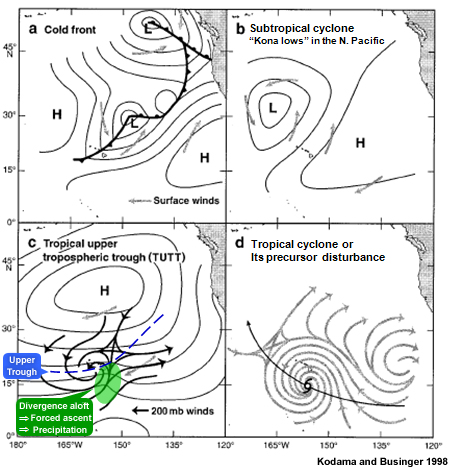
While not as varied or as strong as midlatitude synoptic weather systems, synoptic weather systems are common to many parts of the tropics. For example, the tropical north Pacific is affected by cold fronts and subtropical low pressure systems during the boreal winter, tropical upper tropospheric troughs (TUTTs),35,36 and tropical cyclones and their precursors (Fig. 9.35). Similar systems affect weather in the tropical Atlantic and south Pacific. The Indian subcontinent and Indian Ocean are affected by monsoon low pressure systems, also referred to as monsoon depressions.37,38 Southern Africa experiences dramatic inflow of tropical moisture and heavy rainfall with the passage of tropical-temperate troughs (TTT). 39
TUTTs
TUTTS are semi-permanent summertime features of the Atlantic and Pacific Oceans. Streamline analysis of the 200 hPa winds is a useful tool for identifying TUTTs (Figs. 9.35c and 9.36). Divergence downwind of the TUTT enhances rising motion, low-level convergence, and precipitation (Fig. 9.35c). TUTTs contribute to tropical cyclogenesis where the upper trough location relative to low-level circulation reduces the vertical wind shear. Occasionally, a TUTT will become warm-cored and develop into a tropical cyclone. Learn more about TUTTs in the COMET module, Topics in Tropical Meteorology, http://www.meted.ucar.edu/tropical/met_topics/.
Subtropical Cyclones
These cold-core subtropical cyclones form from the tail-end of midlatitude cyclones during the boreal winter. Over the north central Pacific, they can linger and meander for a more than a week (and, occasionally, weeks).41,42 Typical weather is overcast skies, heavy rains and flooding, severe thunderstorms, and strong winds. Subtropical cyclones over the north Pacific are known as Kona lows because of their association with rainfall over Hawaii.
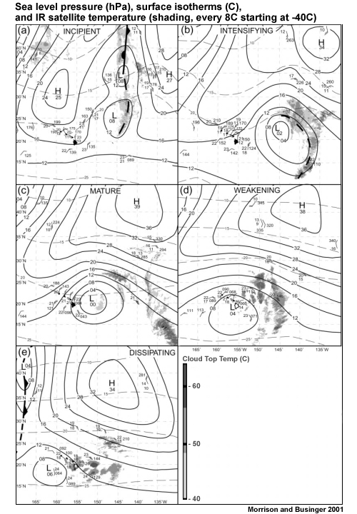
The typical synoptic pattern of a Kona Low is shown in Fig. 9.37; the analysis tools are surface isotherms, sea level isobars, and enhanced satellite IR temperatures. A trough extends equatorward from the low during its early to intensifying stages. Most of the precipitation is on the downstream side of the low pressure center. During the intensifying and mature stages, clouds and precipitation form a comma shape around the surface low. A high strengthens to the north and east of the low. As the cyclone reaches its dissipation stage, the flow around the low becomes more zonal.
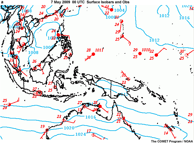
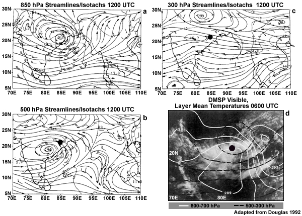
Monsoon depressions are synoptic-scale low pressure systems that are prevalent over the Indian subcontinent and surrounding waters during the summer monsoon.37,38 They last for 3–6 days and typically move west-northwestward at 2–6 m s-1.38 They tilt southwestward with height. Compare the streamline analyses of the surface low location, the 500 hPa cyclone, and 300 hPa trough in Fig. 9.38.43 The heaviest rainfall is usually west of the surface low and the cloud pattern at maturity can resemble weak tropical cyclones (Fig. 9.38d). Many monsoon depressions form from the regeneration of residual low pressure systems that move west from the West Pacific and South China Sea.44 The term monsoon depression has also referred to similar systems that form during the Australian-Indonesian monsoon.
http://www.bom.gov.au/nmoc/MSLP.shtml
Indian Meteorological Department, http://www.imd.ernet.in/main_new.htm
Indonesian Meteorological and Geophysical Agency, http://www.bmg.go.id/
Malaysian Meteorological Department,http://www.met.gov.my/?lang=english
Pakistan Meteorological Department, http://www.pakmet.com.pk/
Singapore Meteorological Service, http://app2.nea.gov.sg/3hnowcast.aspx
Tropical Temperate Troughs
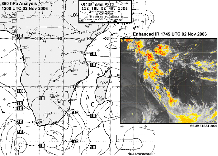
Tropical-temperate troughs (TTT)39 are troughs that connect westerlies with tropical disturbances and brings heavy rainfall to southern Africa. TTTs are summer time phenomena that are somewhat analogous to the semi-permanent SPCZ in the South Pacific and SACZ in the South Atlantic (Fig. 9.31). Generally, a channel of warm, moist air and associated deep convection extends from the NW to the SE as illustrated in Fig. 9.39. One of the signatures of the TTT is strong inflow of tropical moisture by a low-level jet at 850 hPa as seen over along the southern African coast in Fig. 9.39.
Cold fronts
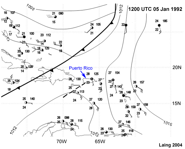
Cold fronts that extend into the tropics do not have a strong temperature gradient; therefore the primary methods used to locate fronts are wind velocity shifts and humidity gradients. Typical winds in advance of the front are from the equatorward side of the front and the air is relatively humid compared with stronger winds and lower humidity on the poleward side. In the Fig. 9.40 example, winds are from the E to SE ahead of the front, and from the NW behind. Kingston, Jamaica is behind the front with dew point at 18°C, while southeast of the front the dewpoint is 24°C although both locations have the same temperature.
How often are tropical regions affected by cold fronts? The number varies by region. For the Dominican Republic, in the northern Caribbean, 15-20% of their winter days are affected by frontal passage; fronts are the primary synoptic weather systems that cause heavy precipitation and thunderstorms during winter.45 The frequency of cold fronts is modulated by interannual oscillations and decadal oscillations. For example, during El Niño winters, strong cold fronts and floods are more frequent across the Caribbean and Central America.46,47 Forecasters should be aware of the climatology of fronts for their region.
Sometimes a surface trough (dashed line in Fig. 9.40) develops in advance of the front and can bring heavy rainfall. These pre-frontal troughs are usually identified from the surface or gradient level wind field; with winds from the equator on the east side of the trough.
Tropical cyclones and tropical easterly waves
Tropical cyclones are the deadliest tropical weather systems (Chapter 8). They form over the warm, tropical oceans; therefore synoptic analysis of tropical cyclones relies heavily on satellite observations because standard meteorological observations are sparse over the oceans. Ships and aircraft rightly avoid tropical storm tracks. Routine in situ observations are only available from reconnaissance aircraft over the Atlantic and East Pacific. Research aircraft also provide data during field projects. As described in Chapter 8, the surface wind field is analyzed from scatterometer measurements while cloud drift winds provide information on flow around the cyclone. Microwave images from LEO satellites provide details of the cloud and precipitation structure once or twice per day. Tropical easterly waves are precursors of tropical cyclones (Chapter 8, Section 8.3.3.1). Time-height plots of wind velocity and moisture are useful for tracking easterly waves (e.g., Fig. 9.24).
Tropical cyclones are the deadliest tropical weather systems (Chapter 8). They form over the warm, tropical oceans; therefore synoptic analysis of tropical cyclones relies heavily on satellite observations because standard meteorological observations are sparse over the oceans. Ships and aircraft rightly avoid tropical storm tracks. Routine in situ observations are only available from reconnaissance aircraft over the Atlantic and East Pacific. Research aircraft also provide data during field projects. As described in Chapter 8, the surface wind field is analyzed from scatterometer measurements while cloud drift winds provide information on flow around the cyclone. Microwave images from LEO satellites provide details of the cloud and precipitation structure once or twice per day. Tropical easterly waves are precursors of tropical cyclones (Chapter 8, Section 8.3.3.1). Time-height plots of wind velocity and moisture are useful for tracking easterly waves (e.g., Fig. 9.24).
You can explore tropical cyclones in depth in Chapter 8. We will review methods of tropical cyclone prediction and validation in Sections 9.5 and Section 9.6, respectively.
You can explore tropical cyclones in depth in Chapter 8. We will review methods of tropical cyclone prediction and validation in Sections 9.5 and Section 9.6, respectively.
Unified Surface Analysis, http://www.opc.ncep.noaa.gov/Loops/#Unified_Surface_Analysis_Products
Regional and Global Analysis, Australian Bureau of Meteorology,
http://www.bom.gov.au/nmoc/MSLP.shtml
9.3 Weather Analysis »
9.3.4 Synoptic-scale Analysis »
Box 9-2 Operational Procedure for Synoptic Weather Analysis
While specific analysis tasks may be automated or manual, the following procedure is common to most forecast centers. Weather analysis has been enhanced by the ability to animate, zoom, create cross sections, do rapid combinations of different fields, and to create derived products. Manual methods yield some of that information by overlaying each weather field on a transparent chart on a light table or by analyzing each field with a different colored pencil on the same map.
Climatology and Planetary-scale Circulations
- Forecasters should be aware of monthly climatology for their area.
- Examine the current ENSO and MJO assessment and forecast. See if local area is in a favorable location for decrease or increase in precipitation due to passage of the MJO.
Surface and Gradient Level charts
- Plot all current observations on weather map (a few hours may be plotted to supplement current observations, e.g., Fig. 9B2.1).
- Examine satellite images (mainly IR, visible), animate geostationary images for previous 12-24 hrs.
- Identify boundaries such as fronts or the ITCZ with the appropriate symbols.
- Strive for consistency and continuity with the previous forecast; make incremental adjustments.
- Analyze pressure field (1-2 hPa interval for the tropics, except for tropical cyclones where larger intervals are necessary).
- Animate pressure analysis for synoptic hours from previous day (for continuity/trends).
- Refine current pressure analysis and boundary positions based on supplemental data such as winds or precipitation from LEO satellite images received within past 3 hrs.
- Analyze streamlines and isotachs based on point and satellite observations.
- Overlay streamlines on satellite images and animate to refine analysis.
- Where available, overlay analyzed divergence/convergence contours.
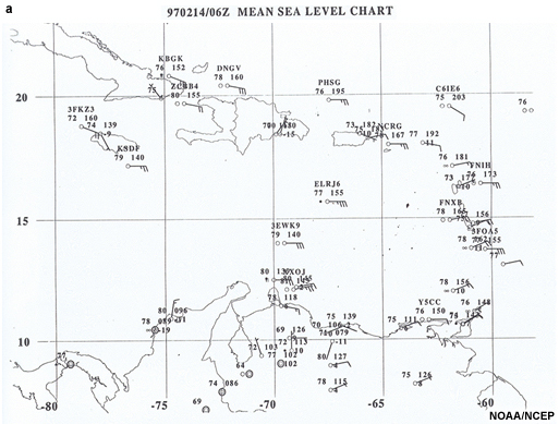
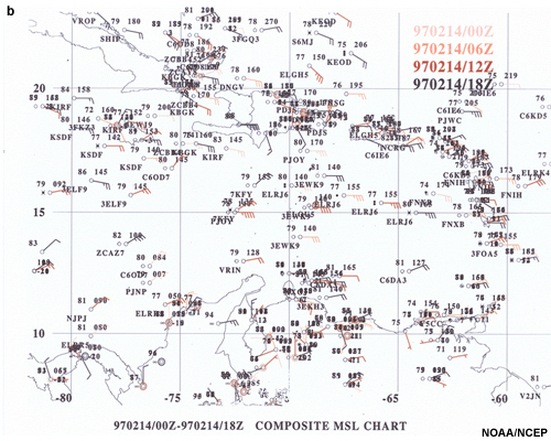
Upper-Level charts
- Plot all current observations on your weather map.
- Examine satellite images (water vapor, enhanced IR, visible), animate geostationary images for previous 12-24 hrs (every hour).
- Analyze geopotential height field (10 dam interval for the tropics, except for tropical cyclone where larger intervals are necessary).
- Analyze streamlines and isotachs based on point and satellite observations.
- Overlay streamlines on water-vapor satellite images and animate to refine analysis of synoptic features.
- For 250 and 200 hPa, overlay divergence/convergence on streamline analysis.
- For 850 hPa, analyze the equivalent potential temperature to help identify heavy rainfall and severe weather potential.
http://www.hpc.ncep.noaa.gov/international/intl2.shtml#charts
http://www.hpc.ncep.noaa.gov/discussions/fxca20.html
http://www.hpc.ncep.noaa.gov/discussions/fxsa20.html
http://www.hpc.ncep.noaa.gov/international/scs/Columbia4.html
9.3 Weather Analysis »
9.3.5 Mesoscale and Convective-scale Analysis
As mentioned at the start of this chapter, tropical weather is dominated by local and mesoscale effects rather than by synoptic influences (except for tropical cyclones and even there the core and rainbands are mesoscale features). Summer and winter weather systems over the Caribbean are used to demonstrate some mesoscale analysis and nowcasting techniques such as satellite analysis, radar interpretation, and surface meteograms.
9.3 Weather Analysis »
9.3.5 Mesoscale and Convective-scale Analysis »
9.3.5.1 Satellite-based Mesoscale Analysis
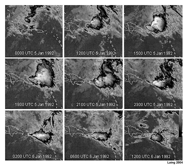
Mesoscale analysis begins with diagnosis of the synoptic regime. First, we look at a winter weather case that included a cold front and pre-frontal trough (shown in Fig. 9.40). We know that these systems usually bring rain to a large area. But how will the rainfall intensity vary within that large area? How will rainfall evolve at the mesoscale?
Enhanced satellite IR images are used to identify mesoscale convective systems (MCSs). First, we identify the most intense convection from the coldest cloud tops, the white areas in Fig. 9.41. Next, we examine the shape and evolution of the convective features. Between 0000 and 1800 UTC on 5 January, the cloud tops are becoming colder. In addition, many more cold clusters are forming and moving southward over the northeastern Caribbean islands. After 1800 UTC, the area of cold cloud decreases but the convection increases in intensity, changes shape, and expands westward. By 0200 UTC 6 Jan, the coldest clouds are aligned in an east-west pattern with an apex formation to the west. An apex point formation in the enhanced IR image indicates back-building (new cells forming upstream of the old cells). When new cells form and track over the same location as the old cells, the result is saturated ground, increased runoff, and flash floods. The ensuing flash flood was one of the worst recorded in Puerto Rico (23 deaths and 88 million US dollars in damage).23
The synoptic diagnosis shows support for MCS formation over Puerto Rico; the surface trough and approaching cold front (Fig. 9.40), the inflow of high θe air at 850 hPa (Fig. 9.23a), and a deep layer of moisture and uplift (Fig. 9.23b). The satellite IR imagery provides the mesoscale details that indicate the flash flood potential. Given the significant impact of these kinds of large MCSs, it is easy to see why it is critical to identify their satellite signature.
![]() Why should tropical weather forecasters be alert to small mesoscale and convective-scale systems?
Why should tropical weather forecasters be alert to small mesoscale and convective-scale systems?
To help answer that question, we will now explore summer weather events over the Caribbean. We will use a case identified by Kathy-Ann Caesar of the Caribbean Institute for Meteorology and Hydrology.
With synoptic-scale features such as Tropical Storm Gustav over the east central Caribbean and an associated trough over the eastern Caribbean, and the ITCZ (Fig. 9.42a), it is tempting to ignore other, smaller weather systems (Fig. 9.42b,c).
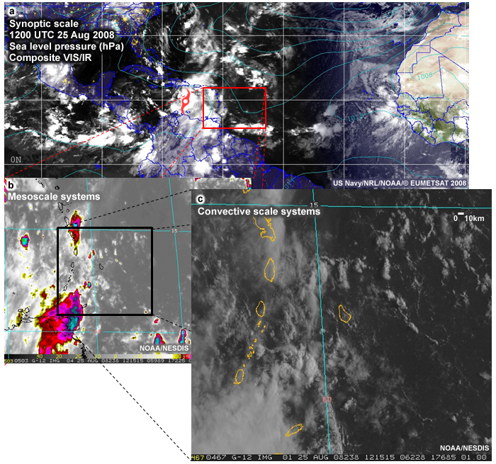
Rain bands move from south to north across the islands following the flow into Gustav. However, Gustav's rain bands are not the only source of precipitation on 25 August. Confluence along the ITCZ and inflow into Gustav (Fig.9.43) leads to the formation of an intense mesoscale convective system (MCS, Fig. 9.42b) over Venezuela and Trinidad and Tobago. As we move down to smaller spatial scales (Fig. 9.42c), we notice narrow bands of clouds to the east of the MCS. How do these cloud bands fit into the precipitation picture on this day?
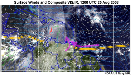
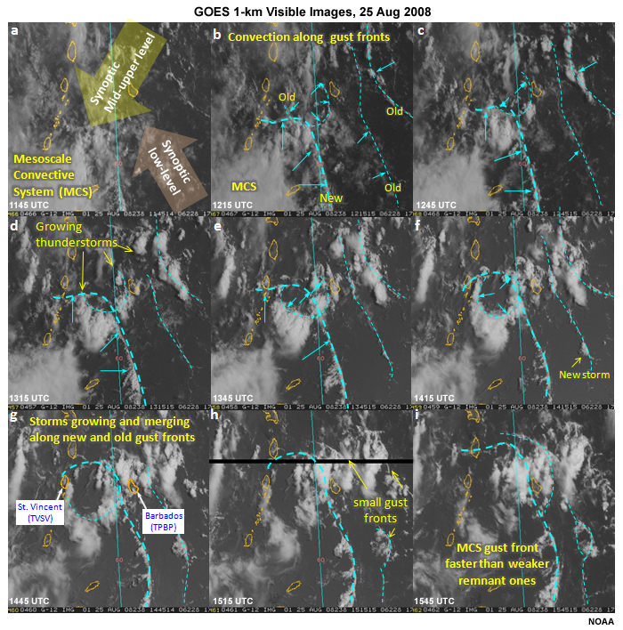
Figure 9.44 shows the merging of an eastward moving thunderstorm gust front and southeasterly cloud bands over the eastern Caribbean. With a strong mesoscale system over the southern Caribbean during the morning (Fig. 9.42b, Fig. 9.44a), the formation of a strong gust front is not surprising. This gust front remained well defined over a long distance—indicating that the downdrafts generated by the MCS were relatively cool. In fact, Piarco Airport in Trinidad experienced a 3°C drop in temperature with the onset of moderate rain and thunderstorms (Fig. 9.45). For forecasters in the neighboring islands, frequent high-resolution, geostationary satellite images are the only available means of tracking the narrow cloud bands associated with gust fronts over the ocean.
These thunderstorm outflow boundaries are different from cloud lines that form along synoptic shear lines over tropical oceans. The latter often form perpendicular to an abrupt change in the horizontal wind, last for several days, and move with the synoptic flow. Gust front duration is on the order of hours and their pattern will match flow emanating from existing thunderstorms.
Returning to the question asked earlier, why should tropical weather forecasters be alert to small mesoscale and convective-scale systems? We will use surface meteograms (Fig. 9.45) to help us analyze the time evolution of the systems seen in the satellite images. (Type your response in the box below.)
Feedback:
Over the humid tropics, and especially over the warm ocean, even small, converging cloud lines can create sufficient updraft for moderate precipitation (Fig. 9.45). As shown in these meteograms, a few hours after the MCS gust front moved away from Trinidad, it converged with weaker gust fronts moving westward and with clouds lines moving in synoptic southeasterly flow. The result was moderate to heavy showers over St. Vincent and light to moderate showers over Barbados (Fig.9.45b,c). At Arnos (Kingstown), St. Vincent, winds shifted from easterly to southerly with the passage of the gust front. Convection over and around Barbados was initiated along several converging thunderstorm gust fronts (Fig. 9.44d-i). For tropical regions with little radar coverage, 1-km visible images from geostationary satellite can provide sufficiently high resolution for local storm monitoring and nowcasting.
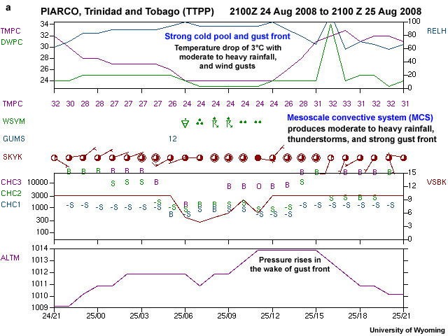
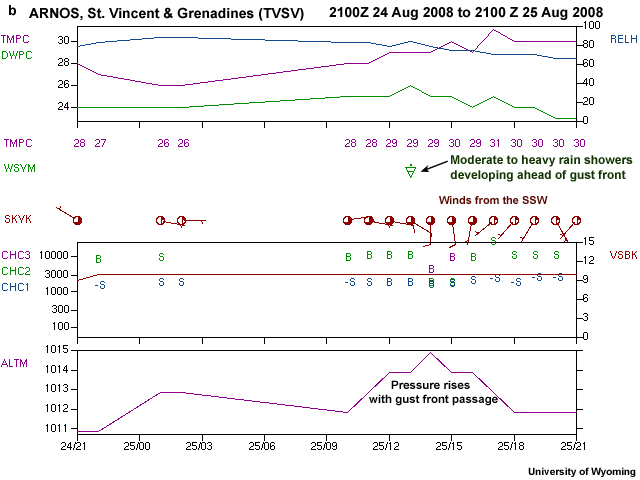
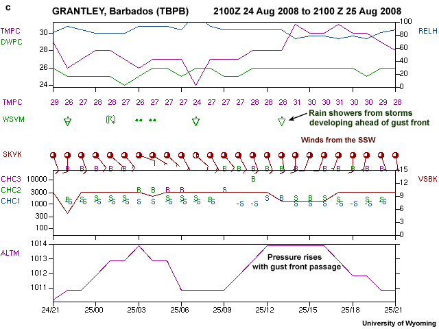
9.3 Weather Analysis »
9.3.5 Mesoscale and Convective-scale Analysis »
9.3.5.2 Radar-based Mesoscale and Convective-scale Analysis
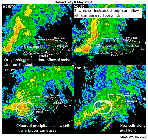
Radars enhance forecasters’ ability to monitor and forecast mesoscale and convective-scale phenomena. We will use the Puerto Rico floods of 6 May 2001 (Fig. 9.36) to illustrate. Synoptically, a TUTT produces a broad precipitation band. But, the mesoscale structure and intensity of the precipitation is varied (Fig. 9.46). Radar analysis shows the impact of the island on the precipitation band. As the large precipitation band moves closer to Puerto Rico, the heavy precipitation line breaks into smaller multi-cellular structures. The northern part becomes weaker and more stratiform. By 1700 UTC, the line has two bow echoes along the west coast, critical features to monitor because they can produce swaths of damaging, straight-line surface winds. The most intense cells are concentrated over the southwest. From 1800 to 2200 UTC, the heaviest precipitation is oriented almost west to east with new cells forming to the west and moving along a similar track as older cells. After 2300 UTC, the intense cells are again aligned along a SW-NE line. Other interesting features, revealed by the radar, are lines of new cells forming in advance of the main band of precipitation, indicating uplift along thunderstorm outflow boundaries. An example can be seen at 2303 UTC. Animation of the radar images also shows bands of precipitation to the north of the island oriented from SE to NW and moving towards the northeast.
9.4 Numerical Weather Prediction in the Tropics
9.4 Numerical Weather Prediction in the Tropics »
9.4.1 Fundamentals of Numerical Models
Numerical prediction models are ubiquitous in modern weather forecasting. The theoretical basis for numerical weather prediction (NWP)48 is dynamical meteorology, which provides the equations that describe the evolution of the atmosphere. Dynamic forecasting predicts the future state of the circulation using numerical approximations of the dynamic equations.
The first attempt at NWP was made by British scientist, L.F. Richardson, who, in 1922, described a procedure for approximating the equations of motion as algebraic difference equations that could be computed for a finite set of grid points. An initial state would be extrapolated forward over a short period to give future estimate. Richardson’s experiment failed to make a decent forecast, in part because of Lamb waves (acoustic waves), dominating the solution. Using the complete equations can create problems, so that filtering the equations (while less accurate in an absolute sense) keeps the meteorologically significant solutions. Richardson estimated that a team of 64,000 people would be needed for a global system of numerical forecasts. His vision has since been realized by high-speed digital computers and a myriad of NWP models categorized by:
- Scale (micro, meso, synoptic, global)
- Application (e.g., general circulation model, dispersion and transport model)
- Dimension (1D, 2D, etc…), and
- Physical assumptions (e.g., hydrostatic or non-hydrostatic).
9.4 Numerical Weather Prediction in the Tropics »
9.4.1 Fundamentals of Numerical Models »
9.4.1.1 Basic Conservation Principles and Equations
NWP models represent the behavior of the atmosphere that is described by the primitive equations or governing equations:
- The Momentum Equations
Newton’s second law of motion stated as the force balance for acceleration relative to a rotating coordinate frame. The horizontal momentum equation can be stated as,where (5)
(5) is the horizontal velocity vector (m s-1), t is time (s),p is pressure (Pa), f is the Coriolis parameter (s-1), ρ is density (kg m-3),
  is the sum of gravitational and centrifugal forces, Fr is friction and turbulent mixing. D/Dt represents the sum of the local rate of change plus advection terms. The horizontal wind is a primary weather variable. The acceleration of the horizontal wind is on the order of 10-4 m s-2 compared with 10-7 m s-2 for the vertical acceleration,
Primitive equation models assume that horizontal scales are much larger than vertical scales, which applies to synoptic and planetary circulations. The vertical momentum equation is replaced by the hydrostatic approximation, in which the weight of the atmosphere balances the vertical pressure gradient. No vertical accelerations are calculated explicitly,
is the sum of gravitational and centrifugal forces, Fr is friction and turbulent mixing. D/Dt represents the sum of the local rate of change plus advection terms. The horizontal wind is a primary weather variable. The acceleration of the horizontal wind is on the order of 10-4 m s-2 compared with 10-7 m s-2 for the vertical acceleration,
Primitive equation models assume that horizontal scales are much larger than vertical scales, which applies to synoptic and planetary circulations. The vertical momentum equation is replaced by the hydrostatic approximation, in which the weight of the atmosphere balances the vertical pressure gradient. No vertical accelerations are calculated explicitly, (6)
(6) , and
, and
 (7)However, the hydrostatic assumption does not hold when the length and depth are similar (typically ≤ 10 km). Deep convection, which is common in the tropics, is non-hydrostatic. Hydrostatic models try to account for buoyancy in deep convection by parameterizations (Section 9.5). Non-hydrostatic models explicitly forecast buoyancy and its effects. Therefore, the rate of change of vertical motion is calculated as the sum of the advection, local buoyancy, and non-hydrostatic vertical pressure gradient minus the precipitation drag. These models can reproduce mesoscale convection in realistic detail but they are subject to error in timing and placement of convection. Non-hydrostatic models have the disadvantage of being computationally intensive.
However, the hydrostatic assumption does not hold when the length and depth are similar (typically ≤ 10 km). Deep convection, which is common in the tropics, is non-hydrostatic. Hydrostatic models try to account for buoyancy in deep convection by parameterizations (Section 9.5). Non-hydrostatic models explicitly forecast buoyancy and its effects. Therefore, the rate of change of vertical motion is calculated as the sum of the advection, local buoyancy, and non-hydrostatic vertical pressure gradient minus the precipitation drag. These models can reproduce mesoscale convection in realistic detail but they are subject to error in timing and placement of convection. Non-hydrostatic models have the disadvantage of being computationally intensive.
- The Continuity Equation
A fundamental principle in meteorology is that mass is conserved except for external sources and sinks, as described by the equation,which can be rewritten as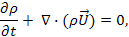 (8) where
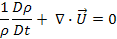 (8a) is the velocity, t is time, and ρ is density. The second form of the equation is useful for forecasting as it relates the rate of density increase, following an air parcel, to the velocity divergence.
- The Thermodynamic Equation or First Law of Thermodynamics
This equation describes the conservation of energy applied to a moving fluid element. For a system in thermodynamic equilibrium, the change in internal energy is due to the difference between work done by the system and heat added to the system, written as:The first term is the change in internal energy per unit mass, cv is the specific heat at constant volume (717 J kg -1 K-1), T is temperature (K). The second term is the rate of work by the fluid system per unit mass, α is specific volume (1/ρ), p is pressure, and Q is heating rate. We can rewrite the thermodynamic equation as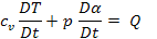 (9)where cp is the specific heat at constant pressure. For adiabatic processes no heat is exchanged with surroundings. Therefore any work done in the system is taken from the internal energy and the temperature decreases.
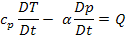 (10)
(10)
Two kinds of atmospheric motion and time scales can be defined in the primitive equations:
- The inertial time scale,
 , where f is the Coriolis parameter.
 - The advective time scale,
 , where LH, the horizontal length scale far exceeds the vertical scale and VH is a typical horizontal velocity.
Usually, for the atmosphere, the advective time scale is more than one day while the inertial time scale is a few hours, τ2 » τ1. Inertial-gravity waves have time scales < τ1, and speeds well in excess of VH. Advective motions are of primary meteorological significance, especially for the synoptic-scale, except near and above the tropopause where inertial-gravity waves have a significant role. Also, in the tropics f is small; therefore the time scale of inertial-gravity waves is close to other motions and is not as easy to separate. Nevertheless, for the most part, inertial-gravity waves are a minor component of the flow, the noise that is undesirable in numerical prediction models. Learn more about the primitive equations in the COMET module, Model Fundamentals, http://www.meted.ucar.edu/nwp/model_fundamentals/.
9.4 Numerical Weather Prediction in the Tropics »
9.4.1 Fundamentals of Numerical Models »
9.4.1.2 Grid Point Models
All models begin with a system of coupled differential equations. Consider a simple example of a two-dimensional advection equation
 (11)
(11)where q is any continuous scalar variable, such as temperature, U is constant, t is time, x, and y are distance and the three are continuous.
To solve for q numerically, we consider t, x, and y as discrete dimensions. A continuous field can then be represented by model grid points (e.g., Fig. 9.47).
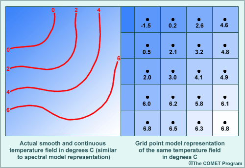
The advection equation can be approximated by a finite difference equation, the simplest form of discretization. The analytic solution is approximated by a Taylor series. The centered difference form of the equation involves points at equal distances on either side of the forecast point:
 (12)
(12)The predicted value of q at time, t+∆t, is
 (13)
(13)Figure 9.48 illustrates the conceptual form of the equation,
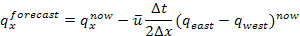 (14)
(14)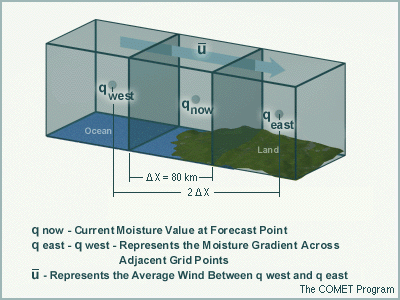
Models also use forward and backward difference techniques to calculate the predicted value. Given current and historical values of the variable, q, we can calculate its future values. By repeating the process with continual addition of new data for a prescribed period, we obtain a numerical forecast.
If the difference equations are not stable, if parts of the numerical solution are unbounded, then the numerical solutions will grow exponentially. The stability of a centered difference numerical scheme can be measured by the Courant-Friedrichs-Levy (CFL) criterion,
 (15)
(15)where c is the speed of the fastest wave in the system. To avoid computational instability, a decrease in the time step requires a decrease in the grid spacing so that the variables are advected less than one grid length per time step. Other forms of finite differencing techniques may require stricter criteria.
9.4 Numerical Weather Prediction in the Tropics »
9.4.1 Fundamentals of Numerical Models »
9.4.1.3 Spectral Models
Spectral models represent the atmospheric spatial variability as a finite series of sine and cosine waves of differing wavelengths. Model resolution is a function of the number of waves that are used to represent variability in the model. Several types of wave orientation are possible in spectral models. The wave length of the smallest number in a spectral model is represented as

The T170 configuration is commonly used in operational models because its resolution in the zonal and meridional directions is almost the same around the globe. Although horizontal gradients are calculated exactly from the wave solution, grids are still used for non-linear and physical calculations. Spectral models are the primary models at operational forecast centers such as ECMWF and NCEP, while grid point models are used for smaller, regional models.
9.4 Numerical Weather Prediction in the Tropics »
9.4.1 Fundamentals of Numerical Models »
9.4.1.4 Vertical Coordinate
Some models use pressure as the vertical coordinate because the primitive equations are simpler on pressure surfaces. The disadvantage is that some pressure surfaces will be below ground. A terrain following or sigma (σ) coordinate avoids those problems and allows representation of high resolution above complex terrain. Sigma ranges from 0 to 1 and is defined as,
 (16)
(16)where ps is the ground level pressure and p is the variable pressure. Other models use isentropic surfaces, equal potential temperature surfaces, along which potential vorticity is conserved. The advantage is that synoptic-scale vertical motion can be easily diagnosed on isentropic surfaces but they intersect the surface and they are poor representations of the boundary layer, especially during the daytime. They are better at resolving frontal boundaries and the tropopause.
Many current models use a hybrid sigma-pressure coordinate, with sigma coordinates near the surface and pressure coordinates near the top.49 Sigma-isentropic hybrid coordinate systems are formulated similarly. Most models have variable vertical resolution with highest resolution usually in the boundary layer. This is especially important for pollutant dispersion models where vertical mixing and wind shear in the boundary layer are critical. Learn more about model vertical coordinates from the COMET Module, Impact of Model Structure and Dynamics.
9.4 Numerical Weather Prediction in the Tropics »
9.4.1 Fundamentals of Numerical Models »
9.4.1.5 Model Forecast System
A conceptual diagram of a model forecast system is presented in Fig. 9.49. Operational models are typically run at six hourly synoptic intervals (0000, 0600, 1200, 1800 UTC).
Initialization and Data Assimilation
Models are initialized with data from the global observation network (Section 9.2.1). The spatial and temporal resolution of the phenomena of interest determines the model configuration. “Resolution” is a term commonly used to refer to grid spacing but they are different. At least four grid boxes are needed to resolve a feature. Therefore a model with 20 km grid spacing will depict features of 80 km or greater!
During initialization, model equations are filtered to remove mechanisms responsible for exciting unwanted oscillations such as inertial-gravity waves and sound waves. To create the model initial conditions, a data “assimilation” procedure incorporates observations of the atmosphere over a limited time period (typically hours) to express the current state of the atmosphere in a framework that the model can use. More details are presented in the next section, Section 9.4.2.
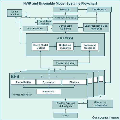
Forecast model
The type of model, computational capacity, and application dictates the choice of numerical formulation, dynamics, physical approximations, and data assimilation procedure. For operational models, efficiency is balanced with accuracy in order to produce timely forecasts. Global model forecasts are provided from 6 hours to 14 days in advance. However, the skill rapidly decreases beyond seven days for synoptic-scale variables such as the 500 hPa geopotential height in midlatitudes. For clouds and precipitation, the skill is considerably less.50
Post processing
After the model run is completed, post processing tools are used by the forecaster to derive specific variables of interest such as 500 hPa geopotential height, amount or type of precipitation. The forecaster adjusts the model predictions based on his or her knowledge of the regional climatology, model biases, and recent weather in order to create forecasts for specific user communities. For example, model analysis is combined with observations to diagnose zones of confluence and severe weather over southern Africa (Fig. 9.50) and, consequently, model forecasts are used to identify zones of severe weather and heavy rainfall for the following day (Fig. 9.51).
Verification
Forecast systems are evaluated systematically in order to test their skill and identify biases. Verification identifies deficiencies and help developers to improve the model. Verification techniques are described in detail in Section 9.6.
Forecast systems are evaluated systematically in order to test their skill and identify biases. Verification identifies deficiencies and help developers to improve the model. Verification techniques are described in detail in Section 9.6.
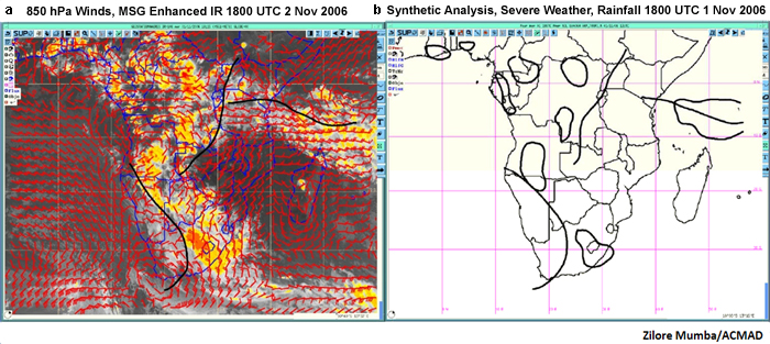
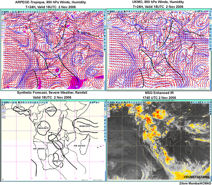
Limited Area Models
Limited area models or regional models nested within global models are run operationally and for research. A list of commonly-used regional models is provided in Table 9.1. Regional models are being applied to aviation, agriculture planning, military operations, response to hazardous chemical release, and hydrometeorology, to name a few. While regional models provide high resolution, they are bounded by the lateral boundary conditions from the global models. Those lateral boundary conditions are sources of error, e.g., errors can be created by the numerical techniques used to interface the two different model scales.51 High resolution models will depict more realistic features but those features are highly likely to be inaccurate in position and timing.
| Global Operational Numerical Weather Prediction Systems | |
| National Centers for Environmental Prediction
(NCEP) Global Forecast System (GFS) |
http://mag.ncep.noaa.gov/NCOMAGWEB/appcontroller |
| NCEP Ensemble Products (Experimental) |
http://www.emc.ncep.noaa.gov/gmb/ens/ |
| NOAA Operational Model Archive Distribution System (NOMADS) |
http://nomad3.ncep.noaa.gov/ http://nomads.ncdc.noaa.gov/data.php |
| Navy Operational Global
Atmospheric Prediction System (NOGAPS) |
http://www.nrlmry.navy.mil/metoc/nogaps /nogaps_char.html |
| European Centre for Medium-Range Weather Forecasts (ECMWF) |
http://www.ecmwf.int/products/ |
| Canadian Meteorological Centre, Global Environmental Multiscale (GEM) model |
http://collaboration.cmc.ec.gc.ca/science/rpn/gef_html_public/index.html |
| United Kingdom (UK) Met Office Unified Model and Met Office Short-range Ensemble System (MOGREPS) |
http://www.metoffice.gov.uk/weather/world/ http://www.metoffice.gov.uk/research/areas/data-assimilation-and-ensembles/ensemble-forecasting/MOGREPS |
| Meteo-France Action de Recherche Petite Echelle Grande Echelle (ARPEGE) Global Model |
http://www.cnrm.meteo.fr/gmapdoc/ |
| Examples of Operational and Real-time Limited Area Models used in the Tropics | |
| NCEP North American Mesoscale Model | http://mag.ncep.noaa.gov/NCOMAGWEB/appcontroller |
| Weather Research and Forecasting (WRF) Model | http://www.wrf-model.org/plots/wrfrealtime.php http://www.wrf-model.org/ |
| Advanced Research WRF (ARW) | http://www.wrf-model.org/plots/realtime_main.php |
| WRF Nonhydrostatic Mesoscale Model (WRF-NMM) |
http://www.dtcenter.org/wrf-nmm/users/ |
| Naval Research Laboratory, Coupled Ocean/Atmosphere Mesoscale Prediction System (COAMPS) |
http://www.nrlmry.navy.mil/coamps-web/web/home |
| Australian Bureau of Meteorology, LAPS (Limited Area Prediction System) and TXLAPS (Tropical eXtended Area Prediction System) |
http://www.bom.gov.au/nmoc/NWP.shtml |
| Indian Meteorological Department Limited Area Model forecasts |
http://www.imd.gov.in/section/nhac/dynamic/welcome.htm |
| China, Regional Service Guangzhou | http://www.grmc.gov.cn/ |
| Hong Kong Observatory Operational Regional Spectral Model (ORSM) |
http://www.hko.gov.hk/nwp/nwpe.htm |
| Aire Limitée, Adaptation dynamique, Développement InterNationale (ALADIN- Réunion Limited Area Model) |
http://www.meteo.fr/temps/domtom/La_Reunion/meteoreunion2/ |
| Brazilian National Institute of Meteorology (INMET) |
http://www.inmet.gov.br/ |
| Caribbean Institute for Meteorology and Hydrology (CIMH) |
WRF,
http://63.175.159.26/~wrf/?pageID=2sAdft&content=wrf MM5, http://63.175.159.26/~mm5/?pageID=2sAdft&content=mm5 |
| Deutscher Wetterdienst High–resolution Regional Model (HRM) |
http://www.met.gov.om/hrm/memb.html |
| NOAA WaveWatch III (WW3) |
http://polar.ncep.noaa.gov/waves/pres/primer /primer_1.html |
Marine Forecasting Models
Wave models use winds and near surface temperature forecasts from atmospheric models and SST analyses52 as input. Most use the statistical properties of waves to predict the sea state at a point,53 rather than trying to predict individual waves. Models predict the energy spectrum of these waves over a range of discrete frequencies and directions. A wave action density equation is used to relate the frequency and direction of wave energy to the sources and sinks of wave energy. The sources and sink terms are parameterized based on studies of physical processes such as the dissipation of energy during wave breaking.
Adjustments to the model wave forecast may be necessary when the marine boundary layer become either destabilized or stably stratified. When warm air moves over cold water, the marine boundary layer becomes strongly stratified, winds aloft are decoupled from the surface, and model wave heights may be over-predicted. When cold air moves over warm water, the boundary layer is destabilized, winds accelerate, and model wave heights are likely to be under predicted.
For information on current operational models, see COMET module, Operational Models Matrix: Characteristics of NWP and Related Forecast Models, http://www.meted.ucar.edu/nwp/pcu2/marine_matrix/index.htm
9.4 Numerical Weather Prediction in the Tropics »
9.4.2 Data Assimilation
The aim of data assimilation is to optimize the accuracy of the forecast by blending observations with short range forecasts, also termed the background field. Many observation systems provide data continuously and data assimilation is a way to incorporate those data received between analysis times. The difference between the observation and the background field is called the observation increment or innovation. Data assimilation analyzes the observation increments and creates a grid of “corrections” to the previous short-range forecast (or background field).
(weighted average of observation increments or innovations)
Critical information for data assimilation is the background error covariance, which is the covariance of background error at different points. So, if the model error at one place is usually associated with error at another place, then a correction at the first location implies that the second location also needs correction. A key concept of data assimilation is that weights given to the background and observations are inversely proportional to their error variances; information with smaller error variance (which therefore has smaller expected error) receives larger weight. The combined corrections and short-range forecast form the initial conditions for the next forecast cycle (Fig. 9.52).
Data assimilation procedures are quite complex because observations have different spatial resolution, temporal resolution, and accuracy. The quality of observations varies across observation platform, time of day (e.g., LEO satellite data swaths, radiosonde reports) and weather (e.g., rain contamination of scatterometer-derived winds).
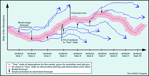
Furthermore, some observations are not the same as model predicted variables, which means that techniques must be developed to relate model analysis and observations. For example, radiances are related to model variables, such as temperature, through radiative transfer equations (Chapter 2, Box 2-1). Predicted radiances are computed from the model state (e.g., temperature, moisture, and ozone profiles) and used to calculate the analysis increments for the background field.
Furthermore, some observations are not the same as model predicted variables, which means that techniques must be developed to relate model analysis and observations. For example, radiances are related to model variables, such as temperature, through radiative transfer equations (Chapter 2, Box 2-1). Predicted radiances are computed from the model state (e.g., temperature, moisture, and ozone profiles) and used to calculate the analysis increments for the background field.
Observation increments are weighted according to perceived accuracy and validity. The weighting given to different pieces of information is based on their error covariance. Data assimilation is complicated by the need for well-behaved computational models for the required error covariances and for good estimates of those covariances. Observation error could be large if the instrument is not very accurate or if the observation network resolution differs from the model resolution. Isolated data in a region of sparse data presents problems for data assimilation as there is nothing to corroborate the observation increment. Errors are also introduced via radiative transfer approximations for satellite radiance assimilation. The flow regime will also affect the quality of the first guess field; error variances will increase in regions of rapid change and decrease in slowly evolving, zonal flow or calm regions. If the first guess field is assumed to be good, then little correction is needed and even perfect observations will show little impact.
In four-dimensional data assimilation (FDDA), new information can be introduced through (i) periodic reanalysis, (ii) gradual insertion (also called dynamic relaxation or nudging), (iii) more advanced mathematical techniques, such as variational four dimensional data assimilation (4DVAR). Variational data assimilation methods include the:
- Three-dimensional variational method, 3DVAR,54,55,56 which uses static background error covariances and seeks to minimize the “distance” between a model solution and available observations. A “distance” or “cost” function,J, is defined as
J= Jb + Jo+ Jc (17)where Jb is a weighted fit of the analysis to the background, Jo is a weighted fit of analysis to the observations, and Jc is used to minimize any noise produced by the analysis. The forecast error covariance functions determine the spreading of observation influence (the inverse error covariance matrix provides the “weighting” in the cost function).
The initial analysis is adjusted for optimal prediction by the “adjoint method”,57,58 which uses an iterative approach. The aim is to find the initial state whereby the corresponding model solution minimizes the function that measures the “distance” between the model solution and the observations. The “adjoint equations” of the model compute the gradient of the distance function with respect to the model’s initial condition. The gradient ensures that the analysis at time, t = 0, is adjusted to provide a better forecast at a future time, e.g., t = 3hr. In 3DVAR only the adjoint of the observation operators (e.g., radiative transfer) are needed.
With 3DVAR, all the points are analyzed at once, using all of the available data. 3DVAR offers the advantages that non-traditional observation types can be included in the analysis, satellite radiance data are used to enhance temperature soundings where data quality and quantity are low (over the tropics, oceans, and Southern Hemisphere), and it optimizes information content from a variety of sensors. One disadvantage of 3DVAR is that background-error covariances are usually assumed to be static (fixed in time) when in reality they may vary substantially with the atmospheric flow of the day.
- 4DVAR method, an extension of 3DVAR that allows a continuous cycle of data assimilation during a specific window of time (typically several hours). It can assimilate asynchronous observations. The initial analysis is adjusted for optimal prediction by the “adjoint method”,57,58 which uses an iterative approach. The aim is to find the initial state whereby the corresponding model solution minimizes the function that measures the “distance” between the model solution and the observations. The “adjoint equations” of the model compute the gradient of the distance function with respect to the model’s initial condition. The gradient ensures that the analysis at time, t = 0, is adjusted to provide a better forecast at a future time, e.g., t = 3hr. In 3DVar only the adjoint of the forward (observation) operators are needed, not the model adjoint. Many operational centers (e.g., ECMWF, France, UK, Japan) use 4DVAR techniques,59 which are more accurate than 3DVAR but more computationally expensive.
Data assimilation is a growing area of weather forecasting as an increasing volume of and variety of data are being incorporated into forecast models. For example, the WRF-Chem model fully integrates both meteorology and chemistry. WRF-Chem explicitly models atmospheric flow and aerosol chemistry and has chemical data assimilation as an experimental option. Only a tiny percentage of available data is currently assimilated into operational models (Fig. 9.6); many are removed prior to using because of redundancy, gross error, or computational expense. Efforts to increase the amount of data assimilated are warranted because satellite data assimilation has improved NWP model performance.11,60,61 For example, ground-based GPS precipitable water vapor, COSMIC GPS refractivity, and standard meteorological observations over the Caribbean have been assimilated into tropical storm forecasts. Explore more in the COMET module, Understanding Data Assimilation: How Models Create Their Initial Conditions, http://www.meted.ucar.edu/nwp/model_dataassimilation/.
9.4 Numerical Weather Prediction in the Tropics »
9.4.3 Sources of Model Forecast Errors
9.4 Numerical Weather Prediction in the Tropics »
9.4.3 Sources of Model Forecast Errors »
9.4.3.1 Initial Conditions
The model initial analysis combines a variety of observations (while accounting for differing resolution and accuracy) and the first guess field of the model, which must be consistent with the model resolution and physics. Errors are introduced when observations are sparse and/or infrequent. The initial state may not be realistic because of errors in the observations themselves (e.g., instrument error or lack of representativeness) which are then transmitted to the objective analysis and data assimilation. Errors are also introduced in interpolating the first guess field to the observation location (the model is forecasting a gridded volume while observations may be at a point).
Forecasters can find out what data are in a particular model run by overlaying satellite images, analysis, and raw data. Then they can see inconsistencies caused by data sparseness, wind perturbations from gust fronts, or features too small or fast-moving for the model to predict. Forecasters should become aware of situations in which the assimilation system is more likely to fail and to pay attention to evolving weather in the observations.
9.4 Numerical Weather Prediction in the Tropics »
9.4.3 Sources of Model Forecast Errors »
9.4.3.2 Boundary Conditions
Surface conditions are critical because the model is tuned to respond to surface moisture, land cover, and temperature. The gradients of these values force mesoscale responses, e.g., soil moisture gradients influence where convection develops. Thus errors in the soil moisture will cause errors in the forecast. Furthermore, an unrepresentative surface will affect the surface albedo and subsequent radiation processes.
Regional models are nested within global models, which usually have coarser resolution. The quality of the forecast is potentially degraded because of the differences in horizontal, vertical, and temporal resolution. In addition, errors in the global model forecast can propagate into regional models and contaminate the regional forecast. These errors can be reduced by avoiding strong forcing at the edge of the boundary because the resulting large gradients are not treated realistically, e.g., avoid putting boundaries in complex topography or regions of strong surface temperature gradients. Make a buffer zone between the nested domain and the coarse domain boundary. Interactive nesting, with two-way rather than one-way nesting, should reduce the formation of spurious gradients near the boundaries.51
It is important to remember that poor initial conditions can outweigh the benefits of high resolution. Forecasters should check the highest-resolution forecast against later coarse resolution forecasts for the same valid time. If conditions are changing rapidly within the forecast cycles, the larger-scale forcing and boundary conditions may have changed and the coarse-resolution forecast could be better.
9.4 Numerical Weather Prediction in the Tropics »
9.4.3 Sources of Model Forecast Errors »
9.4.3.3 Physical Approximations or Parameterization
The model cannot represent all processes and features that occur within a grid box. Some processes may not be understood well enough to be represented numerically or the data are not available at the scale of interest. The phenomena may be too small or too complex to be resolved numerically. Parameterization is one method of adding the net influence of those processes to the model. It is, arguably, one of the most difficult and controversial area of atmospheric modeling.
Physical processes such as water phase changes, radiation, and turbulence in the boundary layer are usually parameterized and referred to as the “physics” of the model. In most models, each process is parameterized separately. However, the model evolves according to their combined effect. It is difficult to diagnose model error associated with each separately. An error in one parameterization may be nurtured by another parameterization and their effect may be compounded at different model resolutions. For example, the vertical distribution of temperature and water vapor content are affected by how convection is coupled to the surface processes. Errors in predicting or diagnosing the presence of clouds produce large errors in short- and longwave radiation calculations. The shapes of cloud particles, whose growth is prescribed by a particular microphysical scheme, also affect radiation fluxes.
Model performance and organization of precipitating systems are sensitive to the microphysics, which control grid-scale clouds and precipitation, through latent heat release distribution and radiative feedbacks.
Turbulence and friction in the boundary layer are sensitive to the prescribed roughness length, which may introduce errors in the forecast winds, vertical wind shear, and consequently to the fluxes of heat, moisture that are transported upward. Errors in emulating surface processes are caused by incorrect surface energy and/or water balances in the model. Certain assumptions, such as the profile of diffusion rate in the PBL, may introduce errors. Learn more about physical assumptions in the COMET module, Influence of Model Physics on NWP Forecasts, http://www.meted.ucar.edu/nwp/model_physics/index.htm.
9.4 Numerical Weather Prediction in the Tropics »
9.4.3 Sources of Model Forecast Errors »
9.4.3.4 Numerical Approximations
Finite difference techniques in grid point models produce truncation errors because they approximate a continuous derivative and higher order derivatives are truncated. Also when equations are integrated over long periods, small-scale noise grows. The error can be reduced by reducing the integration time step.
The shape of the grid also affects the accuracy of the model. The traditional latitude-longitude grids creates problems because the shape of the grid cells becomes more distorted at higher latitudes (Fig. 9.53a), and the discrete approximations become more difficult to implement on multi-processor computer systems. Hexagonal grids have the advantage that cells have nearly equal size and discrete approximations are relatively easy to implement but high-order discretization is difficult. Hexagonal grids and cubed spheres (Fig. 9.53b,c) are being tested for implementation in the next generation of weather prediction models. The computational domain is another source of error. Some grid point models are more difficult to implement on parallel processing systems.
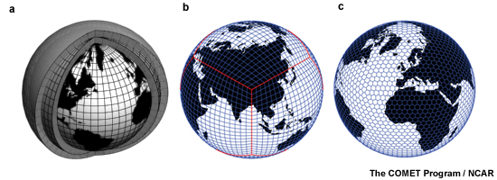
The ability of a model to represent particular phenomena is a function of the size and speed of the features relative to the number of grid points that are needed to sample those features. Grid point models do a poor job of handling waves that are only a few grid points across. Truncation errors occur in spectral models because they only have information for waves that they resolve; smaller scale wave information is not included. Errors occur in spectral models when transformations are made between spectral and grid point physics calculations. In addition, the damping mechanisms used to reduce spurious oscillation during model initialization could adversely affect meteorologically significant motions.
9.4 Numerical Weather Prediction in the Tropics »
9.4.3 Sources of Model Forecast Errors »
9.4.3.5 Intrinsic Predictability
Predictability is intrinsically limited because of the chaotic nature of the atmosphere. Numerous scales of motion exist in the atmosphere and energy transfers among them. Energy from scales smaller than the resolution of the observations is not in numerical models. Therefore, the real atmosphere and the model atmosphere are different. Over time, the numerical forecast and the real atmosphere will diverge (Fig. 9.54). Any error in the initial condition or in the model will cause a loss of predictability.62 Even small differences in initial conditions can lead to large errors in a long range forecast. This intrinsic error grows faster at smaller scales than larger scales, which means that small scale weather phenomena are less well forecasted. Predictability limits of small scale phenomena may be as short as 75 minutes for a 20-km wavelength.62,63 Note that chaotic does not mean random but rather we can define a system with a range of possible states (the climate in our case) and predict the evolution of that system with some accuracy for a short period.
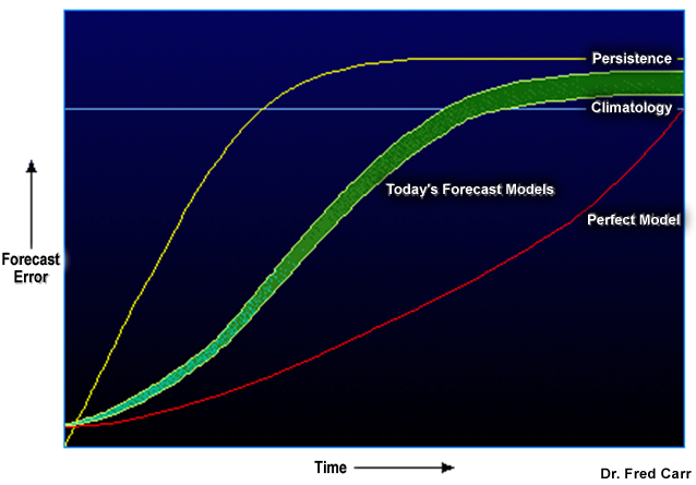
9.4 Numerical Weather Prediction in the Tropics »
9.4.4 Dynamical and Statistical Models
The numerical models described thus far in this chapter are dynamical models; they use the physical laws that govern the behavior of the atmosphere and the ocean to predict their future state. Statistical models or inductive models need past observations in order to predict the future. A long period of record is examined for trends, extremes, and relationships between forecast products and relevant predictors. A basic statistical model would be a simple regression of tropical cyclone central pressure and sea surface temperature (SST). More complex prediction systems use neural networks to train the models to recognize precursor events and predict the probability of forecast outcomes.64,65,66,67 Statistical-dynamical models use statistical relationships between forecast outcomes and predictors from dynamical model forecasts. In Section 9.5, tropical cyclone prediction is used to explore in depth the strengths and weaknesses of dynamical and statistical models.
The numerical models described thus far in this chapter are dynamical models; they use the physical laws that govern the behavior of the atmosphere and the ocean to predict their future state. Statistical models or inductive models need past observations in order to predict the future. A long period of record is examined for trends, extremes, and relationships between forecast products and relevant predictors. A basic statistical model would be a simple regression of tropical cyclone central pressure and sea surface temperature (SST). More complex prediction systems use neural networks to train the models to recognize precursor events and predict the probability of forecast outcomes.64,65,66,67 Statistical-dynamical models use statistical relationships between forecast outcomes and predictors from dynamical model forecasts. In Section 9.5, tropical cyclone prediction is used to explore in depth the strengths and weaknesses of dynamical and statistical models.
9.4 Numerical Weather Prediction in the Tropics »
9.4.5 Ensemble Prediction Systems
A single numerical model produces a specific or deterministic forecast from a specific model configuration (grid spacing, initial conditions, physics, etc.) with its systematic errors. It is possible to measure forecast sensitivity to uncertainty in the model configuration, such as the initial conditions, by perturbing the initial conditions in an NWP model. An ensemble of predictions can then be used to predict uncertainty in the forecast.68,69,70,71,72 Thus, the imperfect nature of initial conditions and NWP models can be used strategically in an ensemble prediction system (EPS) to:
- Establish a range of possible forecast outcomes
- Create members of the ensemble by (i) perturbing the initial conditions, (ii) model dynamics and/or physics, or (iii) model boundary conditions
- Estimate the probability for any individual forecast outcome
- Help to determine the most likely forecast outcome.
Ensembles help to distinguish between weather situations with high or low predictability by tracking how uncertainty in the initial condition will evolve.73 Ensemble means can be better estimates of the expected value of weather variables than a single deterministic forecast. The ensemble spread and higher moments of the forecast probability distribution allows comparison of timing and strength of the perturbations of the ensemble members.
Single-model ensembles have multiple members from the same model and starting time, but using slightly different initial conditions, thereby accounting for the uncertainties in the initial states of the model. Combinations of different models are called multi-model ensembles. For an ensemble forecast to be completed at the same time as an operational deterministic model forecast, the ensemble model usually has lower horizontal resolution. An in-exhaustive list of advantages and weaknesses of ensemble prediction systems is provided in the COMET module, Ensemble Forecasting Explained, http://www.meted.ucar.edu/nwp/pcu1/ensemble/1_1_1.htm.
Regional Ensembles
The NCEP Short-range Ensemble forecast (SREF)74,75 system is the first operational, real-time regional ensemble forecast system. Its ensemble members include one of three dynamical models (Eta model, Regional Spectral Model, WRF), different physical parameterizations (deep convection, boundary layer, radiation, …), one of two different analysis systems, different horizontal and vertical resolution, and perturbations that are bred to sample flow-dependent initial condition error.
9.4 Numerical Weather Prediction in the Tropics »
9.4.5 Ensemble Prediction Systems »
9.4.5.1 Ensemble Output
Different kinds of plots are used to interpret ensemble forecasts. The most common are:
- Spaghetti plots
Plots of contours with each member appear similar to strands of spaghetti, except color-coded for ease of readability. The choice of variables and levels to plot depends on the forecast application, e.g., the freezing level is a critical parameter for aviation. Fig. 9.55a shows the spaghetti plot for the 1012 hPa isobar from NCEP Global Ensemble Forecast System (GEFS). Over the continent, the ensemble members are in very good agreement while over the eastern Pacific, the forecasts are farther apart. For this case, the ensemble forecasts were relatively close to the analysis (Fig. 9.55b).
These plots provide a quick measure of uncertainty (through differences in distance and amplitude among the contours) but are an incomplete picture of the forecast probability distribution. Small differences where the gradient is large can be significant, while large difference where the flow is zonal is of less consequence.
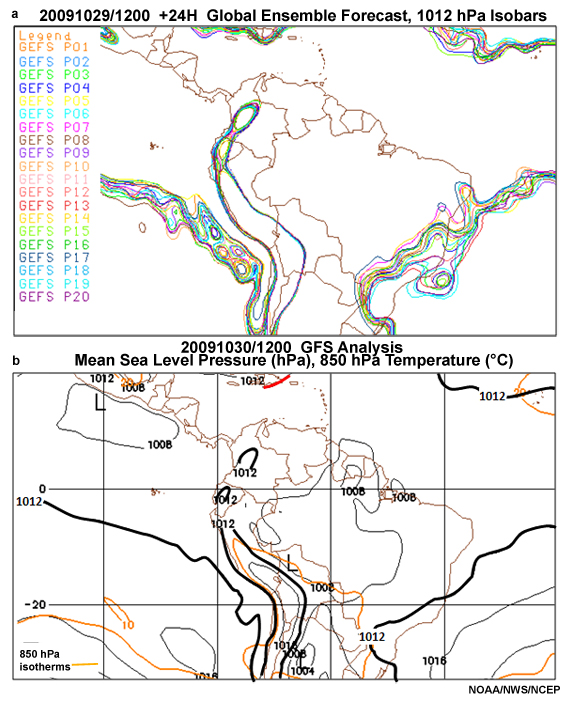
- Ensemble Means and Spread
The mean is the simple average of all ensemble members. The spread is the standard deviation. More spread means more uncertainty in the forecasts. Fig. 9.56 illustrates the interpretation of the mean and spread plots.
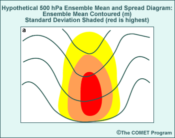
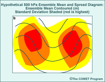
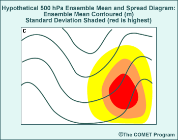
A real case is shown in Fig. 9.57, in which the biggest spread in 850 hPa temperature is found over the South Atlantic Ocean and very little spread over the continent except for northeastern Brazil. The analysis confirms the more skillful forecast over the continental interior, while over the south Atlantic and northeast Brazil, the analysis is very different from the ensemble mean.
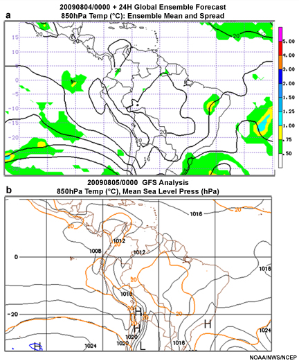
The advantage of the ensemble mean and spread is that a lot of information is summarized in one graph. But, we need to consider that the ensemble mean may not be the best forecast. If clusters of similar forecast outcomes exist, the mean may lie between the clusters.
- Probability of Exceedance Plots
These plots show the probability of the forecast value exceeding a meaningful threshold and are used to identify the probability of extreme events.
- Plume diagram
These are time series of ensemble forecasts from a grid box showing the time evolution of a forecast variable. For example, a plume diagram could show the ensemble forecasts of SST anomaly for the Niño 3.4 region (Fig. 5.51) or the forecast drop in temperature during a cold frontal passage.
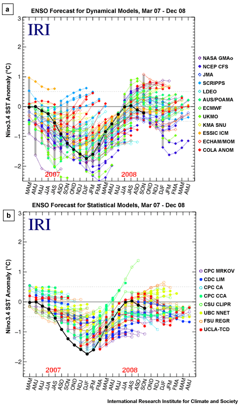
- Ensemble Soundings
Each ensemble member profile and ensemble mean is plotted on a thermodynamic diagram with specific color code.
- Box and Whiskers Diagrams
These show the range of error as a time series (e.g., Fig. 9.58).
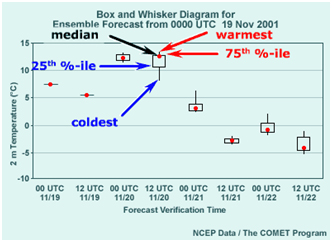
EPS forecasts are verified by comparing forecast probability distributions and other statistics of the EPS to the frequency of observations over time. Therefore a large set of ensemble forecasts, often over an entire season, is needed to obtain stable results. TIGGE, the THORPEX Interactive Grand Global Ensemble (THORPEX: THe Observing system Research and Predictability EXperiment), was established to archive and compare large numbers of operational EPS output.76
http://journals.ametsoc.org/perlserv/?request=get-abstract&doi=10.1175%2FMWR2949.1
NCEP Ensemble Training,
http://www.hpc.ncep.noaa.gov/ensembletraining/
9.4 Numerical Weather Prediction in the Tropics »
9.4.5 Ensemble Prediction Systems »
9.4.5.2 Ensemble Data Assimilation
For ensemble modeling systems, a commonly used data assimilation technique is Ensemble Kalman Filter (EnKF).77,78 EnKF uses ensembles to determine the error statistics associated with the first guess field of the model. Unlike 3DVAR (Section 9.4.2), for which error statistics are isotropic and stationary, ensemble-based error statistics have flow dependence and can adjust to the unique flow of the day. The ensemble transform Kalman filter (ETKF) is a specific form of the EnKF that has the advantage of being fast, suitable for generating ensemble initial conditions, and updating perturbations of the initial conditions. However, it does not represent sampling error efficiently.79 The ETKF has been used to select flight tracks and target deployment of dropwindsondes for tropical cyclone surveillance.80 Data assimilation by variational, ensemble, and hybrid techniques have relative merits and weaknesses for operational forecasting.81,59 Hybrid variational and EnKF data assimilation systems are being tested to better handle data that involves highly non-linear processes such as clouds and precipitation. For instance, the WRF hybrid system82 combines ensemble covariances and 3DVAR covariances, both climatological and flow-dependent estimate of the background error statistics.
You can learn more about ensemble forecasting in the COMET module, Ensemble Forecasting Explained, http://www.meted.ucar.edu/nwp/pcu1/ensemble/)
9.4 Numerical Weather Prediction in the Tropics »
9.4.6 Cumulus Convection in NWP
Cumulus convection is ubiquitous in the tropics and latent heat transport in cumulus convection is the primary method of transferring energy from the surface to the atmosphere. Therefore, cumulus convection needs to be represented in numerical models of tropical weather. As illustrated Fig. 9.59, cumulus convection occurs at several scales, which means that it is impossible to predict individual clouds. Therefore, numerical models create parameters to account for the effect of cumulus convection within a given grid box.
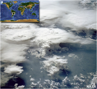
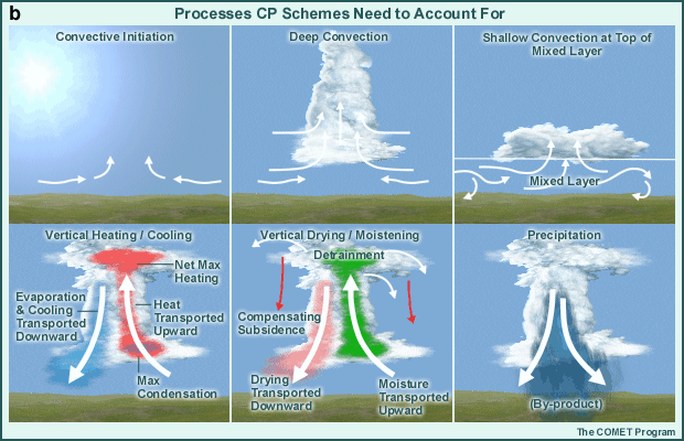
Cumulus parameterization schemes try to account for many processes, including the vertical transports of heat, moisture, and momentum by convective updrafts and downdrafts; some of these processes are illustrated in Fig. 9.59b.
A summary of approaches to cumulus parameterization in mesoscale models83 is presented in Table 9.2. Models with sufficiently small grid spacing to resolve mesoscale circulations (less than 5 km grid spacing in the midlatitudes) can be run without cumulus parameterization. Instead precipitation is produced using explicit microphysics at each grid point. With the traditional approach, grid-scale precipitation is produced by cumulus parameterization, the implicit method. Other models use a hybrid of the two approaches.
Approach |
Convectively unstable points |
Convectively stable points |
| Traditional | Implicit | Explicit |
| Fully Explicit | Explicit | Explicit |
| Hybrid | Hybrid | Explicit |
While cumulus parameterization provides a quick way to represent the effects of convection, their use can be problematic.84 Sometimes parameterization schemes produce convection at the wrong time or less/more intense than observed. The split of precipitation between grid scale and cumulus parameterization schemes for a given system depends on the choice of scheme and model resolution.85 How models treat the crossover between cumulus parameterization and explicit microphysics and how the processes are activated and weighted affect the distribution of heating in the modeled convective systems. Cumulus parameterization schemes experience difficulties simulating propagating convection;86 perhaps because they are not specifically designed to simulate propagation as they act independently in individual model columns.87 Comparison of the quality of one convective parameterization scheme versus another is difficult because forecast skill is a function of the complete model including the interaction of different physical parameterizations and other sources of error (Section 9.4.3).
While cumulus parameterization provides a quick way to represent the effects of convection, their use can be problematic.84 Sometimes parameterization schemes produce convection at the wrong time or less/more intense than observed. The split of precipitation between grid scale and cumulus parameterization schemes for a given system depends on the choice of scheme and model resolution.85 How models treat the crossover between cumulus parameterization and explicit microphysics and how the processes are activated and weighted affect the distribution of heating in the modeled convective systems. Cumulus parameterization schemes experience difficulties simulating propagating convection;86 perhaps because they are not specifically designed to simulate propagation as they act independently in individual model columns.87 Comparison of the quality of one convective parameterization scheme versus another is difficult because forecast skill is a function of the complete model including the interaction of different physical parameterizations and other sources of error (Section 9.4.3).
Below are characteristics of three convective parameterization schemes often used for tropical weather prediction (conceptual models of two of them are shown in Fig. 9.60). For a more complete list and detailed description of current convective parameterization schemes, see the COMET module, http://www.meted.ucar.edu/nwp/model_precipandclouds/.
- Arakawa-Schubert:84 Requires that convective stabilization be in balance with large-scale destabilization rate, accounts for moisture detrainment from clouds, and warming from subsidence. Convection is triggered by some CAPE in the boundary layer, minimum cloud depth and maximum CIN are specified.
- Betts-Miller-Janjic:88 Adjusts the model sounding toward a pre-determined, post-convective reference profile derived from climatology. Convection is triggered by a moist sounding with some CAPE and cloud depth exceeding a threshold.
- Kain-Fritsch:89 Rearranges mass within an atmospheric column so that CAPE is consumed during convection. Convection is triggered by CAPE from a lower tropospheric layer that is 50-100 hPa thick (sub-cloud layer); where warm, moist air is capped by an inversion small enough for a parcel to penetrate with only a few m s-1 of vertical speed; and when the convective cloud depth exceeds a threshold.
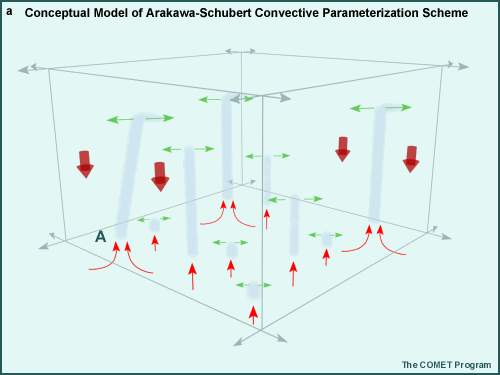
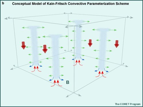
With advances in computer power, very high resolution models are now being run operationally. While models do not predict individual clouds, models with grid spacing of less than 5 km can resolve mesoscale cloud features.90,91,92 However, while convection permitting 2-km grid models produce detailed convective activity, they had little forecast skill on the scales where those details appear.50 Therefore it may not be worth the computational cost to implement operational models with such high resolution.
Cloud resolving models (CRMs) were developed as one method of modeling the complex interactions among cloud microphysics, cloud dynamics, radiation processes, and surface processes in tropical cumulus. CRMs explicitly resolve the dynamical circulations that directly couple these various physical processes. They were first applied to modeling convection in climate models.93 In recent years, computational advances have facilitated “superparameterization”, a process that combines conventional cumulus parameterization on a coarse grid with detailed cloud-resolving modeling on a finer grid. The effects of moist convection are expressed through explicit turbulent fluxes.
http://www.meted.ucar.edu/nwp/model_precipandclouds/print.htm#page_3.0.0
NOAA Geophysical Fluid Dynamics Laboratory, Mesoscale Dynamics,
http://www.gfdl.noaa.gov/visualizations-mesoscale-dynamics
Cumulus parameterization on the mesoscale,
http://www.bom.gov.au/bmrc/basic/wksp15/Dare.pdf
Ten Common NWP Misconceptions,
http://www.meted.ucar.edu/norlat/tencom/index.htm
9.5 Tropical Cyclone Prediction
Accurate forecasts of tropical cyclone (TC) evolution rely first on having an effective conceptual model that incorporates the key physics of this evolution. These physics must be accounted for in NWP models used by forecasters. Because all forecast models have some weaknesses, we need effective ways of evaluating model forecasts to identify their good and bad points. With this knowledge, forecasters can integrate all of the possible futures given by the different models and produce the most skillful forecast. We will explore each of these facets here.
9.5 Tropical Cyclone Prediction »
9.5.1 Factors that Influence Motion and Intensity
9.5 Tropical Cyclone Prediction »
9.5.1 Factors that Influence Motion and Intensity »
9.5.1.1 Factors Contributing to Tropical Cyclone Motion
Tropical cyclone motion is predominantly governed by the steering flow of its environment. The steering flow is the net effect of the winds from all of the other weather systems that affect the tropical cyclone. Since tropical cyclones extend through many kilometers, with the most intense of them reaching up to the tropopause, we must consider the winds through this whole layer when calculating the steering flow.
If steering were all that was important, we could think of a tropical cyclone like a cork in a river and things would be simple. But a tropical cyclone is much more complicated: it is comprised of hundreds of thunderstorms, all growing and dying constantly, and held together by the storm’s wind field. The structure of the tropical cyclone means that other factors affect its motion.
After steering, one of the most vital factors contributing to tropical cyclone motion is the “β-effect” (Chapter 8, Section 8.7.1). The β-effect describes how tropical cyclone motion is affected by the Coriolis parameter due to the Earth's curvature. The asymmetric flow resulting from the vortex interacting with the Coriolis parameter is known as β-gyres.
After steering, one of the most vital factors contributing to tropical cyclone motion is the “β-effect” (Chapter 8, Section 8.7.1). The β-effect describes how tropical cyclone motion is affected by the Coriolis parameter due to the Earth's curvature. The asymmetric flow resulting from the vortex interacting with the Coriolis parameter is known as β-gyres.
Since the β-gyres rely only on the tropical cyclone and the Earth’s vorticity (Coriolis), the tropical cyclone will move due to the β-gyres, even if there is no steering flow. Typically, propagation due to the β‑gyres adds 2–5 m s-1 to the speed and is directed poleward and westward of the storm. Therefore, a storm at 20°N would propagate towards the northwest, while a storm at 20°S would propagate to the southwest. Using vector addition, we calculate tropical cyclone motion due to steering flow and propagation due to the β-gyres (Fig. 9.61).
Since the β-gyres result from advection of varying background vorticity, if the environment of the tropical cyclone has relative vorticity gradients of similar magnitude to β, we need to include these in calculating the storm propagation. However, because the relative vorticity due to other weather systems could have gradients in any direction, the direction of propagation is not known ahead of time.
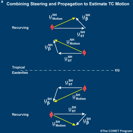
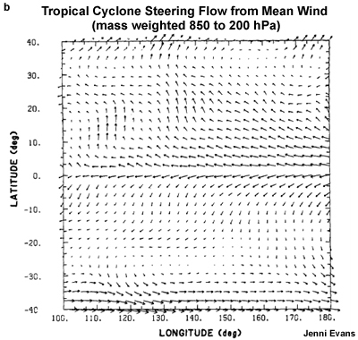
Other factors affect the motion of a tropical cyclone: tropical cyclone structure and intensity, as well as the vertical shear of the environmental winds and the presence of other weather systems. The tropical cyclone structure governs the size and strength of the β-gyres, so the propagation of two tropical cyclones at the same latitude, but with different structures, will be different.
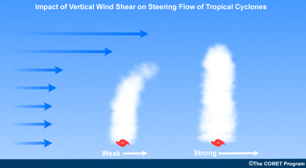
The intensity of the tropical cyclone is linked to the vertical extent of the storm. Stronger tropical cyclones have more vigorous thunderstorm activity and are generally taller than weaker tropical cyclones. This means that we need to calculate the steering flow through a deeper layer for a strong tropical cyclone than a weak one (Fig. 9.62).
The vertical wind shear can change motion since the average wind through the depth of the tropical cyclone is the steering flow. It can also affect the motion in another way; if the wind shear is too strong, the tropical cyclone will weaken and its structure will change.
The presence of other tropical cyclones influences storm motion because the two storms will steer each other— known as the “Fujiwhara effect”—and results in the two storms circling each other (Fig. 8.62). Since tropical cyclones are smaller than the majority of synoptic weather systems, the Fujiwhara effect might be masked by both storms also being advected by other weather systems. To determine whether the Fujiwhara effect is operating, we subtract off the average motion of the two storms, and then plot their motion relative to this larger steering flow. The relative motion for Hurricane Iris (1995) and Tropical Storm Karen (1995) is plotted in Fig. 9.63. This example illustrates that a strong TC can absorb a weaker TC. The stronger system absorbs the weaker one through the very strong horizontal wind shear of its rotating flow. Hurricane Luis and Tropical Storm Jerry also impacted Iris and Karen. This was an atypically crowded period in the North Atlantic! Hurricane Luis and Tropical Storm Jerry also impacted Iris and Karen. This was an atypically crowded period in the North Atlantic!
The presence of other tropical cyclones influences storm motion because the two storms will steer each other— known as the “Fujiwhara effect”—and results in the two storms circling each other (Fig. 8.62). Since tropical cyclones are smaller than the majority of synoptic weather systems, the Fujiwhara effect might be masked by both storms also being advected by other weather systems. To determine whether the Fujiwhara effect is operating, we subtract off the average motion of the two storms, and then plot their motion relative to this larger steering flow. The relative motion for Hurricane Iris (1995) and Tropical Storm Karen (1995) is plotted in Fig. 9.63. This example illustrates that a strong TC can absorb a weaker TC. The stronger system absorbs the weaker one through the very strong horizontal wind shear of its rotating flow. Hurricane Luis and Tropical Storm Jerry also impacted Iris and Karen. This was an atypically crowded period in the North Atlantic! Hurricane Luis and Tropical Storm Jerry also impacted Iris and Karen. This was an atypically crowded period in the North Atlantic!
Clearly the environmental factors affecting motion are linked with each other and with the intensity of the TC. Next we will look briefly at the factors affecting intensity.
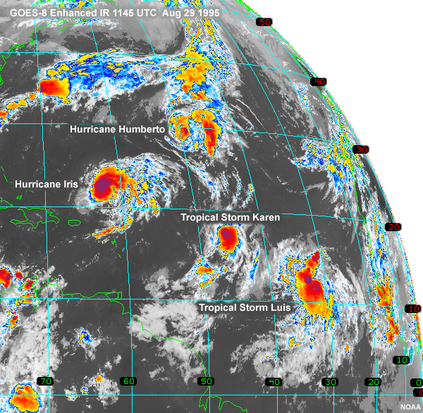
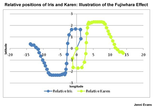
9.5 Tropical Cyclone Prediction »
9.5.1 Factors that Influence Motion and Intensity »
9.5.1.2 Factors Affecting Tropical Cyclone Intensity Change
The environment of the storm (vertical wind shear, ocean temperatures, relative humidity, other weather systems) and its own current structure and intensity affects its future intensity. The key to a storm maintaining its current intensity or intensifying further is the maintenance of the deep convection surrounding its core.
The warm tropical ocean provides the moisture to drive the convection, increasing the moist static energy of the TC boundary layer. Conversion of this moist static energy (Chapter 5, Section 5.2.3) into kinetic energy via convection is the mechanism by which a tropical cyclone intensifies, therefore cool SST or dry air intrusion should lead to weakening of the TC. Theories for the potential intensity (PI) of TC focus on the thermodynamics of the storm (Chapter 8, Section 8.4.1). However, very few TC ever attain their PI, so we need to think about the environment and thermodynamics of the TC.
As mentioned earlier, strong vertical wind shear can weaken a TC; the storm structure adjusts to the new, sheared, environment (Fig. 9.64). The environmental wind shear will induce convection on the downshear side of the storm. The downshear convection will initially create an asymmetry in the eyewall; the storm has to regain the symmetry in the core before it can intensify further. Depending on the structure and intensity of the TC, it may reintensify once the convection gets reorganized and the eyewall regains it symmetry, or it may recurve – then either undergo extratropical transition (potentially reintensifying as an extratropical cyclone; Chapter 8, Section 8.5), or decay.
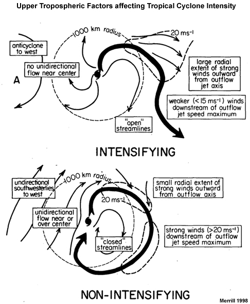
What is it about the storm structure that can change the impact of a given vertical wind shear on a TC? The critical factor is the radius of maximum winds which can change independent of the radius of the 34-kt winds, a common measure of storm size. Intuitively, a rapidly rotating TC with a small radius of maximum winds will be more protected from external influences (such as other weather systems) than a weaker TC with a large radius of maximum winds. We can quantify this difference using inertial stability (Chapter 8, Section 8.2.3.2). High inertial stability makes a storm more resistant to external influences. So a more intense TC can withstand more vertical wind shear than a weaker storm. This means that a stronger TC has the potential to become even stronger unless one of four things happens: 1) it moves over land (rugged terrain will have a stronger impact), 2) it moves over cool water, 3) dry air gets in (via the boundary layer) and weakens the convection in the core, or 4) strong shear in the outflow region of the TC (where inertial stability is weak; Fig. 8.14) shuts off the TC outflow aloft.
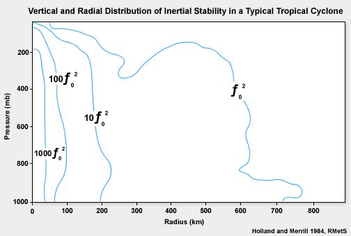
What is it about the storm structure that can change the impact of a given vertical wind shear on a TC? The critical factor is the radius of maximum winds which can change independent of the radius of the 34-kt winds, a common measure of storm size. Intuitively, a rapidly rotating TC with a small radius of maximum winds will be more protected from external influences (such as other weather systems) than a weaker TC with a large radius of maximum winds. We can quantify this difference using inertial stability (Chapter 8, Section 8.2.3.2). High inertial stability makes a storm more resistant to external influences. So a more intense TC can withstand more vertical wind shear than a weaker storm. This means that a stronger TC has the potential to become even stronger unless one of four things happens: 1) it moves over land (rugged terrain will have a stronger impact), 2) it moves over cool water, 3) dry air gets in (via the boundary layer) and weakens the convection in the core, or 4) strong shear in the outflow region of the TC (where inertial stability is weak; Fig. 8.14) shuts off the TC outflow aloft.
In summary, intensity forecasting is a much more complicated problem than track, and indeed it depends strongly on the track (if the TC is forecast in the wrong location, it will experience a different environment). TC intensity depends critically on wind, temperature and moisture patterns in the core of the storm and in the near environment. These are often very challenging to measure and assimilate into models. Intensity change is also governed by internal processes, such as eyewall replacement cycles, that are poorly understood. Intensity change is a multi-scale problem that involves complex interactions between thunderstorms in the TC core and the TC environment, as well as air-sea interactions.
Motion and intensity are not the only important factors needed to forecast the societal impacts of the passage of a tropical cyclone. If we do not know the structure of the wind field – where the strongest winds are and how far out the dangerous winds extend – we are not able to give much guidance to the population. Figure 9.65 shows the dramatic difference in size between Hurricanes Floyd (1999) and Andrew (1992). For example, you might be terrified at the thought that a storm with 40 m s-1 peak winds is headed your way; you may even think of evacuating. However, if you knew that the storm was small enough that you would only experience 10 m s-1 winds – a stiff breeze – you could relax. Conversely, if you knew that this was a really large storm and your house was likely to experience hurricane force winds, you might evacuate to a safe place.
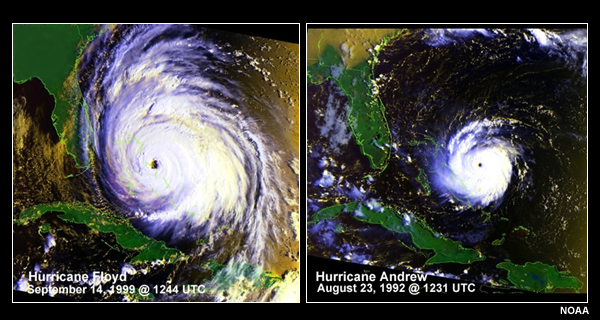
Now that we have the basics of TC evolution, it is time to look at a variety of forecast techniques and methods for deciding which techniques provides the best forecast in a given situation (Spoiler alert: no single technique is the best all of the time)!
9.5 Tropical Cyclone Prediction »
9.5.2 Dynamical Forecast Models Applied to TCs
Dynamical models solve the fundamental physical laws that govern the evolution of the atmosphere and produce a forecast by integrating these equations into the future (Section 9.4.1.1). Clearly then, dynamical models attempt to predict what will happen in a specific situation. This is a key difference between statistical and dynamical models.
The physics of TC motion is generally well understood, relying predominantly on the environmental flow (Sections 8.7, 9.5.1.1) So, track forecasting is relatively straightforward since numerical models have the best skill for synoptic flow. Synoptic weather systems are relatively large and easy to measure and generally evolve slowly (so the model integration will not drift over a given forecast time). Therefore, highly successful track forecasts can be obtained by focusing on the evolution of the storm environment, rather than on the storm itself, a task well suited for dynamical models. A hierarchy of dynamical models of increasing complexity exists and their usefulness varies by situation.
Simplified Dynamical Track Models: Beta and Advection Models (BAMD, BAMM, BAMS)
These “Beta and Advection Models” (BAM) are simple trajectory models that only consider steering and the β-effect on TC motion. In these models, the TC cannot change nor have any impact on its environment.
The three-dimensional wind forecast from a more complex model is averaged in the vertical to create a two-dimensional wind field, the steering flow of the TC. The distinction between BAMD, BAMM, and BAMS is the depth of the layer over which the steering flow is calculated: Deep, Medium, or Shallow. This is the only way that variations in the vertical are incorporated into the BAM motion forecast. The choice of steering layer depends on the intensity of the TC being forecast (see schematic in Fig. 9.64).
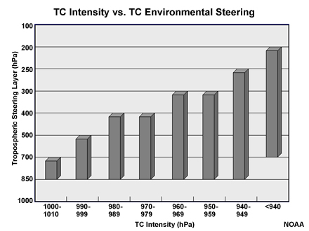
One advantage of the BAM models is their speed. As of 2008, the BAM models run almost instantaneously and so the forecaster can create many forecasts of TC motion, varying the depth of the steering layer and the location of the TC (which can be in doubt, especially for weak systems with indeterminate eye structure). Thus, the forecaster can see how sensitive the forecast could be to these factors and get a sense of the potential for track errors in this situation (Fig. 9.66). Of course, these insights are limited by the lack of consideration of TC evolution and of vertical structure effects.
Global Dynamical (Track and Intensity) Models: ECMWF, GFS, UKMET, NOGAPS
The more complicated, three dimensional dynamical models come in two flavors: Global and Regional. Rather than the single layer of the BAM models, these can include 25-90 layers in the vertical!
Here we briefly review the models available to forecasters at the National Hurricane Center (NHC) in Miami; the main ones used are listed in Table 9.3. Most of these dynamical models are available to all forecast centers. One exception is that the regional (limited area) models will necessarily vary from one region to another. A list of operational limited area models and their applicable regions is given in Table 9.4.
Global numerical models used for TC forecasting have been developed for general NWP (Section 9.4.1.2, 9.4.1.3), not specifically for TC. These models have horizontal resolutions of 25-60 km (e.g., Fig. 9.53). Current global models can usually resolve the general structure of the TC and the synoptic environmental flow and therefore do a good job of predicting tropical cyclone tracks, especially at the longer lead times. However, because of their relatively coarse resolution, the global models cannot represent the TC core structure and are not suitable for intensity prediction.
Global numerical models used for TC forecasting have been developed for general NWP (Section 9.4.1.2, 9.4.1.3), not specifically for TC. These models have horizontal resolutions of 25-60 km (e.g., Fig. 9.53). Current global models can usually resolve the general structure of the TC and the synoptic environmental flow and therefore do a good job of predicting tropical cyclone tracks, especially at the longer lead times. However, because of their relatively coarse resolution, the global models cannot represent the TC core structure and are not suitable for intensity prediction.
| Operational models often used for tropical cyclone forecasting at the U.S. National Hurricane Center | Acronyms | Scale |
NCEP Global Forecast System (GFS) http://www.emc.ncep.noaa.gov/modelinfo NCEP Hurricane Products http://www.nco.ncep.noaa.gov/pmb/products/hur/ |
GFS | Global |
United Kingdom Meteorological Office (UKMET) Model http://www.metoffice.gov.uk/research/modelling-systems/unified-model |
UKMET | Global |
Navy Operational Global Atmospheric Prediction System (NOGAPS) http://www.meted.ucar.edu/nwp/pcu2/nogaps/index.htm |
NOGAPS | Global |
ECMWF Model http://www.ecmwf.int/products/forecasts/guide/ |
ECMWF | Global |
Canadian (CMC) Global Environmental Multiscale Model (GEM), http://www.smc-msc.ec.gc.ca/cmc/op_systems/recent_e.html |
CMC/GEM | Global |
NWS Geophysical Fluid Dynamics Model (GFDL) Hurricane Model http://www.gfdl.noaa.gov/research/weather/tpb_gfdl.html |
GFDL, GFDN | Regional |
Hurricane Weather Research and Forecasting Model (HWRF) http://www.emc.ncep.noaa.gov/HWRF/index.html |
HWRF | Regional |
| Operational models used for tropical cyclone forecasting in different regions | Acronyms | Scale |
Japan Meteorological Agency (JMA) Numerical Models http://www.jma.go.jp/jma/en/Activities/nwp.html |
JMA/GSM | Global |
JMA Typhoon Ensemble Prediction System http://www.jma.go.jp/jma/en/Activities/nwp.html |
JMA/TEPS | Global |
National Meteorological Center of China http://www.nmc.gov.cn/english/product.php?class=hailangdxy |
CNMC | Global |
Australian Bureau of Meteorology, Tropical eXtended Limited Area Prediction System (TXLAPS) http://www.bom.gov.au/nmoc/ab_nmc_op.shtml#TXLAPS |
TXLAPS | Regional |
Regional Dynamical (Track and Intensity) Models: GFDL, GFDN, HWRF
These regional dynamical models have been specifically developed for TC forecasting. Their limited area facilitates higher resolution, but they must cover a large enough domain that the TC will not approach the boundary of that domain. This restriction comes from the numerical treatment of flow near the model boundaries (Section 9.4.3.2). Due to this limited coverage, features far from the TC are not handled as well. This can degrade longer-range forecasts. So, regional models have limited forecast lead time.
These regional dynamical models have been specifically developed for TC forecasting. Their limited area facilitates higher resolution, but they must cover a large enough domain that the TC will not approach the boundary of that domain. This restriction comes from the numerical treatment of flow near the model boundaries (Section 9.4.3.2). Due to this limited coverage, features far from the TC are not handled as well. This can degrade longer-range forecasts. So, regional models have limited forecast lead time.
To achieve the highest possible resolution with the available computer capacity, limited area models typically have multiple layers: a number of finer “nests” exist inside the largest limited area grid. In this way, the model can simulate the atmosphere far from the storm with coarser resolution then increase the resolution near the TC, and increase even more near the TC core. Operational versions of both the GFDL and HWRF models have 9.5 km (6 mile) resolution of their innermost nest; approaching the resolution needed to simulate a realistic eyewall.
Higher resolution means the regional models can potentially do a better job of handling interactions between the tropical cyclone and the environment, which can result in better track and intensity forecasts (e.g., Fig. 9.67, for Hurricane Katrina 2005) at short time range.
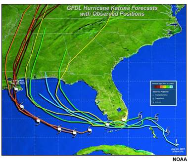
Regional models now have fine enough resolution to begin to simulate the hurricane core (Fig. 9.68), and are capable of predicting rapid changes in intensity. Unfortunately, they do not do so reliably! Presently the dynamical regional model skill is approaching that of the statistical models for intensity. One limiting factor in dynamical forecasts of intensity is the lack of necessary measurements of wind, temperature, and moisture throughout the core and near environment to initialize the models properly. Without these observations, the initial conditions of the model are imperfect, leading to imperfect intensity forecasts.
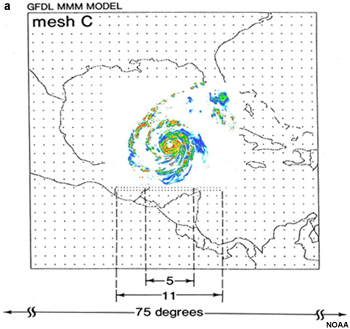
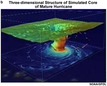
In summary, multi-level regional and global dynamical models are the most skillful models for TC track forecasting. Among these models, the GFDL and GFS have provided the best overall guidance in recent years, but the performance of each model varies significantly from year to year and storm to storm. While it is possible to beat the models from time to time, model performance for track forecasts has improved significantly over the years, and they are very difficult to beat on a consistent basis. Dynamical models cannot as yet out-perform statistical models for intensity forecasting. While neither dynamical nor statistical models can capture rapid intensity changes reliably, dynamical models (in particular, the coupled GFDL model) have shown better, if intermittent, skill.
http://www.nhc.noaa.gov/modelsummary.shtml
How Mesoscale (Limited Area) Models Work,
http://www.meted.ucar.edu/mesoprim/models/index.htm
Hurricane intensity forecast improvements through high resolution models,
http://www.dtcenter.org/plots/hrh_test/HIRES_HFS_Test_Plan.pdf
Features of Current Operational Dynamical Forecast Models
http://www.meted.ucar.edu/nwp/pcu2/index.htm
GFDL Hurricane Visualizations,
http://www.gfdl.noaa.gov/visualizations-hurricanes
9.5 Tropical Cyclone Prediction »
9.5.3 Statistical Forecast Models
Statistical forecast models are based on historical relationships linking a forecast product of interest (motion or intensity) with the behavior of past storms using storm-specific information (i.e., storm location, time of year, current motion, intensity, and environment). The most important thing to remember about statistical models is that they forecast the typical TC behavior in similar situations and do not have skill in forecasting outlier situations such as rapid intensification or sharp track changes. We will now review the statistically-based track and intensity models used at NHC.
Statistical Track Models: CLIPER (Climatology-Persistence)
This is the only statistical model used in forecasting TC track. Since it relies purely on the climatology derived from past storms and on continuing the current TC track, CLIPER knows nothing about the current state of the atmosphere; it simply replicates the typical track for TC in this location, at this time of year, that begin moving in a similar direction. For this reason, CLIPER should not be used as a forecast. However, CLIPER does have one practical application: it is used as a skill baseline to evaluate more complex models. If a track model is not more accurate than CLIPER, it is deemed unusable. After all, if you cannot beat a simple “tomorrow’s track is the average of other TC tracks that were here today” you are in trouble!
Statistical Intensity Models
We have already determined that intensity forecasting is challenging and dynamical models do not yet show reliable skill in forecasting TC intensity—the most skillful intensity forecast models are statistical models. Statistical models merely predict the average behavior of a storm in a given situation. So, our best performing intensity models tell us only what is normal behavior in a particular state. This makes it extremely difficult to forecast unusual or extreme changes in intensity such as occurred with Hurricane Wilma (2005) and illustrated in Fig. 9.69. Statistical intensity forecast models used at the NHC are described below and listed in Table 9.5.
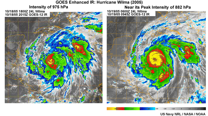
Statistical Hurricane Intensity Prediction Scheme (SHIPS)
SHIPS is a statistical-dynamical intensity model whose forecasts are based on statistical relationships between TC behavior and predictors obtained from dynamical model forecasts.98 SHIPS also includes predictors from satellite data such as the strength and symmetry of convection as measured from IR satellite imagery and the heat content of the upper ocean determined from satellite altimetry observations. Since it includes information about the current state of the atmosphere in addition to climatology and persistence, SHIPS average intensity errors are typically 10%-15% less than the SHIFOR5 errors (See Table 9.5 below).
SHIPS uses multiple linear regression to combine information from the predictors into an intensity forecast. The set of open ocean tropical cyclones from 1982 to the present were used to develop SHIPS; the regression equations are re-derived each year to include TCs from the previous year. This means that the weighting (and so the importance to the forecast) of the predictors can change from year to year. The predictors for SHIPS include:
- climatology and persistence
- atmospheric environmental parameters such as vertical shear and stability
- ocean information such as sea surface temperature (SST) and upper-ocean heat content
The most statistically significant predictors to a skillful intensity forecast are (as of 2008):
- the difference between the current intensity and potential intensity (PI) for this TC
- vertical wind shear
- persistence
- upper-tropospheric temperature
SHIPS has historically outperformed most of the dynamical models, including the GFS which provides the dynamical predictors to SHIPS!
Including information from dynamical models into statistical models can provide increased skill over tropical cyclone forecasts based on current information only. What impact might other approaches, such as ensemble techniques have on tropical cyclone forecasts? We will examine those methods next.
| Statistical Hurricane Model | Summary of Model Characteristics |
| Statistical Hurricane Intensity Forecast Version 5 (SHIFOR5) | Climatology and persistence: The intensity version of CLIPER that is used as a baseline to measure skill in other intensity forecast models. |
| Statistical Hurricane Intensity Forecast with Decay over land (Decay-SHIFOR) | Like SHIFOR, with climatology and persistence, but only for TC over land; a baseline model that provides useful operational intensity guidance. |
| Statistical Hurricane Intensity Prediction Scheme (SHIPS) | Statistical-dynamical model: Uses climatology and persistence plus predictors from dynamical models and satellite diagnostics |
| SHIPS over land (Decay-SHIPS) | Same as SHIPS, but restricted to TC over land. As of 2008, Decay-SHIPS has been the best intensity forecast model on average but it cannot track rapid oscillations. |
| SHIPS Rapid Intensity Index | Same as for SHIPS, but restricted to cases of rapid intensity change (defined as 15 m s-1, 55 km h-1, 35 mph, 30 kt maximum wind increase over 24 hours). It has had mixed success. |
| Logistic Growth Equation Model (LGEM) |
Similar inputs to SHIPS, but more sophisticated statistical approach. |
9.5 Tropical Cyclone Prediction »
9.5.4 Application of Ensemble and Consensus Forecast Techniques
As described in Section 9.4.5, ensemble forecasts are derived from a combination of forecasts; the set of forecasts can either come from multiple models or from an ensemble of forecasts from a single model. A forecast derived by combining a suite of model forecasts is commonly referred to as a consensus forecast (analogous to a group of people reaching a consensus opinion on an issue).
As described in Section 9.4.5, ensemble forecasts are derived from a combination of forecasts; the set of forecasts can either come from multiple models or from an ensemble of forecasts from a single model. A forecast derived by combining a suite of model forecasts is commonly referred to as a consensus forecast (analogous to a group of people reaching a consensus opinion on an issue).
9.5 Tropical Cyclone Prediction »
9.5.4 Application of Ensemble and Consensus Forecast Techniques »
9.5.4.1 Single Model Ensemble Forecasts
Single-model ensembles are from the same model and starting time, but using slightly different initial conditions. The idea is to maximize the spread of the forecasts at a chosen forecast lead time to ensure that the forecast includes the actual (later observed) TC evolution. However, the ensemble runs often have coarser resolution than the deterministic version of the model. This resolution change can introduce differences in the forecast that are not directly related to changes in the initial conditions.
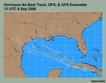
Clearly then, an ensemble forecast could have a very wide range of possibilities (e.g., Fig. 9.70). Often a simple ensemble mean of all of the ensemble forecasts produces a more skillful forecast than any single ensemble run, since errors associated with the individual forecasts tend to cancel each other. However, averaging an ensemble of individual forecasts that tell a very different story—for example, recurvature versus continued westward motion—can result in a forecast that is not very useful (Section 9.4.5). This is where forecasters must use their professional judgment to decide if the ensemble average is meaningful.
Clearly then, an ensemble forecast could have a very wide range of possibilities (e.g., Fig. 9.70). Often a simple ensemble mean of all of the ensemble forecasts produces a more skillful forecast than any single ensemble run, since errors associated with the individual forecasts tend to cancel each other. However, averaging an ensemble of individual forecasts that tell a very different story—for example, recurvature versus continued westward motion—can result in a forecast that is not very useful (Section 9.4.5). This is where forecasters must use their professional judgment to decide if the ensemble average is meaningful.
Here is a summary of ensemble forecast systems often used for TC forecasting:
U.S. National Weather Service Global Ensemble Forecast System (GEFS)
The GEFS is based on the GFS model and consists of a low-resolution (~ 100 km horizontal grid spacing with 28 vertical levels) control run of the GFS, and 20 ensemble members at the same resolution. GEFS produces forecasts out to 16 days, four times per day. TC vortex relocation is applied to the initial conditions of each ensemble member so that the initial TC location is the same in the initial states of all ensemble members.
Meteorological Service of Canada, Canadian Ensemble Forecast System (CEFS)
The CEFS is based on the MSC GEMS model (Table 9.3). GEM is a global grid-point model; the deterministic control run and the 20 ensemble members all have 0.9° x 0.9° (about 100 km x 100 km) horizontal grid spacing and 28 vertical levels. Perturbations representing uncertainties in the initial conditions are developed using the EnKF technique described in Section 9.4.5.2. These perturbations are applied to the control run analysis to create the initial states for each of the 20 ensemble members. CEFS produces forecasts out to 16 days twice per day.
The CEFS is based on the MSC GEMS model (Table 9.3). GEM is a global grid-point model; the deterministic control run and the 20 ensemble members all have 0.9° x 0.9° (about 100 km x 100 km) horizontal grid spacing and 28 vertical levels. Perturbations representing uncertainties in the initial conditions are developed using the EnKF technique described in Section 9.4.5.2. These perturbations are applied to the control run analysis to create the initial states for each of the 20 ensemble members. CEFS produces forecasts out to 16 days twice per day.
The ECMWF Ensemble Prediction System (ECMWF EPS)
The ECMWF EPS has approximately 40 km equivalent horizontal resolution and 62 vertical levels. Its 51 member ensemble, 25 “singular vectors”,99 are developed to generate initial conditions for 50 perturbed forecasts; the deterministic control forecast is the remaining member. These “singular vectors” are measures of forecast differences that will grow most rapidly over time.100 The EPS determines the structure of the initial condition uncertainty tied to these rapidly growing vectors. To include effects of diabatic processes in the region of a TC, moist “tropical” singular vectors101 were introduced into the ECMWF EPS in 2002. Tropical singular vectors are computed in target areas centered on a tropical cyclone of at least tropical storm strength.
Japanese Meteorological Agency Typhoon Ensemble Model (JMA TEM)
The purpose of the Typhoon Ensemble Model is skillful track forecasting. It is a global model with approximately 60 km horizontal grid spacing and 60 levels in the vertical; five day forecasts are run four times per day. The ensemble consists of 11 members. Perturbations are derived using the singular vector approach, which is applied to JMA global model analyses to give the 11 ensemble member initial conditions.
9.5 Tropical Cyclone Prediction »
9.5.4 Application of Ensemble and Consensus Forecast Techniques »
9.5.4.2 Multi-Model Ensembles: Consensus Forecasts
Consensus models are not true forecast models per se, but combinations or averages of forecasts from other models based on the philosophy that two (or many) heads are better than one! Consensus TC models generally outperform the individual models included in them.102,103 Combining the different models allows consensus models take advantage of the fact that model errors are often random. Averaging these different models frequently cancels out these random errors, resulting in a better forecast than any of the individual models. Further, the spread (variation) of individual models making up the ensemble can provide a measure of consensus forecast uncertainty (Section 9.4.5.1).
Consensus models are not true forecast models per se, but combinations or averages of forecasts from other models based on the philosophy that two (or many) heads are better than one! Consensus TC models generally outperform the individual models included in them.102,103 Combining the different models allows consensus models take advantage of the fact that model errors are often random. Averaging these different models frequently cancels out these random errors, resulting in a better forecast than any of the individual models. Further, the spread (variation) of individual models making up the ensemble can provide a measure of consensus forecast uncertainty (Section 9.4.5.1).
The simplest way to form a consensus forecast is to average the output from all model, e.g., one computes the mean of all of the model’s predicted latitudes and longitudes of the TC center at some forecast time. At the NHC, the most commonly-used consensus forecasts are GUNA, CONU, and FSSE, which are described below. Consensus forecasts are typically more accurate (on average) than the predictions from their individual models.
Of course, the consensus approach does not always work, particularly if the model scenarios are completely different. For example, the loops executed by Hurricane Ophelia (2005) off the Florida, Georgia and South Carolina coasts (Fig. 9.71) were not well simulated by most of the models (Fig. 9.69). During the model forecast time Ophelia made a loop off the east coast of Florida.104 The forecast period spanned the time of a subsequent loop off the Georgia and South Carolina coasts on 11-12 September.
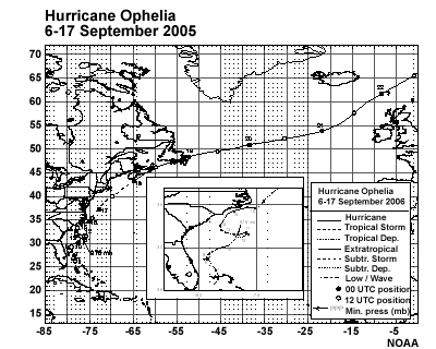
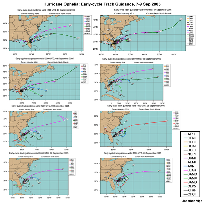
Consensus models available at NHC:
Here we review a few NHC consensus models.97 The consensus models include versions of the primary dynamical models (ECMWF, GFS, UKMET, NOGAPS, CMC, GFDL, GFDN, HWRF) listed in Tables 9.3 and 9.4 Some consensus models include the statistical and statistical-dynamical models listed in Table 9.5
When calculating consensus forecasts, the full suite of models is not always available. However, only some of the consensus products are robust enough to provide a forecast with only a subset of the member models. Sometimes the forecaster may want to exclude certain models and form a “selective consensus”, if the discrepancies among the models can be resolved. However, resolving these discrepancies is very difficult. In Focus Section 2 we learn how forecasters integrate information from models to develop their official forecast.
Even if the forecasters do not make a formal selection of models to use in a consensus forecast, automated “corrected consensus” models produce both track and intensity forecasts. A corrected consensus forecast uses past performance of the member models to reach an optimal combination (subset) and/or to correct the biases of these models to derive the most skillful forecast possible. Specific constituents of each consensus model are available from the NHC.97
Consensus TC Intensity Models: An example
ICON: Decay-SHIPS, GFDI, HWRF, LGEM
ICON was introduced in 2008. It is an intensity consensus forecast computed as the equally weighted average of the Decay-SHIPS, GHMI (adjusted GFDI forecast), HWRF and LGEM intensity output. It has the advantage of including two statistical and two dynamical models, which brings an additional degree of independence to the forecast approach.
Consensus TC Track Models: Examples
GUNA, CGUN: GHMI, EGRI, NGPI and GFSI
The GUNA track consensus forecast is an average of four models: GHMI, EGRI, NGPI and GFSI.a All four member models must be available and all models receive equal weight. CGUN is GUNA corrected for the individual model biases. The model bias corrections are derived statistically using parameters known at the start of the forecast, such as model spread, initial intensity, location, etc.
TVCN, TVCC: GFDI, GFNI, NGPI, UKMI, GFSI, HWFI, EMXI
TVCN is the uniformly weighted average of the guidance from seven models but only a subset (at least two) is required to produce a forecast. Its members are evaluated each year and may vary from year to year. TVCC is the bias corrected version of TVCN.
Consensus TC Track and Intensity Models: An example
Florida State University Super Ensemble: FSSE
The Florida State University Super Ensemble (FSSE) is a weighted multi-model consensus that uses the previous official NHC forecast and the dynamical model members from the other consensus models. Individual model biases are based on the past performance of each member model using a training database made up of approximately 75 sets of past forecasts from each model. The FSSE assigns different weights to each member model. These weights are determined using linear multiple regression during the 75 forecast set training phase. FSSE is somewhat different from other models used at NHC because it is constantly learning from the past performance of its constituent models.
One limitation of the FSSE occurs when the past performance of the member models does not accurately represent their present performance. For example, if major changes were made to a member model between successive hurricane seasons the FSSE may under- or over-estimate the skill of that model. Thus, the FSSE technique is most accurate when no major changes are made to any of the member models between the training phase and operational forecast phase.
Prediction of Track Error: Goerss Prediction of Consensus Track Error (GPCE)
The GPCE provides a measure of the uncertainty in the consensus track forecast105 that is better than the standard approach based on forecast skill for previous storms.105
How does GPCE do it? Intuitively, you might expect a large spread in the model forecasts could lead to large forecast uncertainty and potentially large track errors. Also, differences at the initial forecast time also point to uncertainties that could affect the forecast. Following this logic, Goerss produced this predicted consensus error product which depends on a combination of:
- consensus model spread (difference between each ensemble member and the ensemble average for a chosen metric, e.g. latitude, longitude, intensity )
- initial and forecast TC intensity
- initial TC location
- forecast displacement of TC location (latitude and longitude)
- TC speed of motion, and
- number of members available (for TVCN).
Using these predictors and actual TC behavior for the 2002-2006 seasons, stepwise linear regression models were found to predict the consensus TC track forecast error for each combination of forecast length and consensus mode (Fig. 9.73).
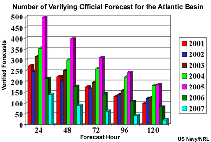
The regression models were then used to determine the radii of circular areas drawn around the consensus model forecast positions within which the verifying TC position was expected to be approximately 75% of the time.
The regression line between the GCPE calculated 120-hour forecast error and the error in the 120 h consensus track forecast is plotted in Figure 9.74. To be sure that the consensus track error is smaller than the GCPE predicted forecast error at least 75% of the time, the regression line is adjusted upwards so that it no longer intersects at the origin. As a result, this adjusted regression gives you 75% “confidence circles” around consensus forecast.
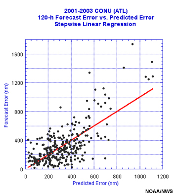
So how did this work? For the 2007 Atlantic season, the circles displayed by GPCE (Fig. 9.75) contained the verifying TC position 72%, 71%, 76%, and 83%, of the time at 24 h, 48 h, 72 h, 96 h, and 120 h, respectively (Fig. 9.76). Therefore if you took notice of the circle, not just the lines, you would have been ready for the storm at least 71% of the time.
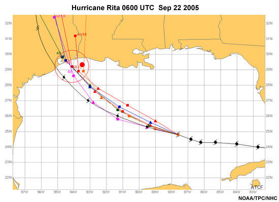
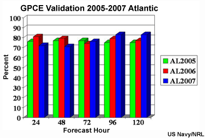
How well do the consensus track models perform?
Ensemble and consensus forecasts take more effort to produce than any of the member models. So are they worth it? Comparison of the relative forecast skill of commonly used consensus models with their member models and the official forecast (Fig. 9.77) provides insight into the added value of consensus forecasting. In Fig. 9.77, verification statistics for 12–120 h track forecasts from the GUNA, CONU and FSSE consensus models are compared against their member models (GFSI, GFDI, GFNI, UKMI and NGPI) and the official (OFCL) NHC forecast. Skill is measured as percentage improvement relative to the corresponding CLIPER forecasts (Section 9.5.3). These skill statistics were calculated from all available North Atlantic storm forecasts from the 2004–2007 hurricane seasons.
Ensemble and consensus forecasts take more effort to produce than any of the member models. So are they worth it? Comparison of the relative forecast skill of commonly used consensus models with their member models and the official forecast (Fig. 9.77) provides insight into the added value of consensus forecasting. In Fig. 9.77, verification statistics for 12–120 h track forecasts from the GUNA, CONU and FSSE consensus models are compared against their member models (GFSI, GFDI, GFNI, UKMI and NGPI) and the official (OFCL) NHC forecast. Skill is measured as percentage improvement relative to the corresponding CLIPER forecasts (Section 9.5.3). These skill statistics were calculated from all available North Atlantic storm forecasts from the 2004–2007 hurricane seasons.
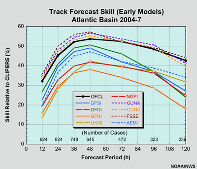
We see that the multi-model consensus forecasts have greater skill overall than either the single GFS model ensemble average (AEMI) or any of the individual models (Fig. 9.77). However, the weighted consensus forecasts (FSSE) do not substantially improve on the simple unweighted average consensus forecasts (GUNA and CONU).
At first glance, Figure 9.77 looks puzzling. Why should the skill be worse for 12 hour and 24 hour forecasts than the later forecasts, even out to 96 hour lead time? (Type your answer in box.)
Feedback:
The problem is not that the forecast models being worse at short (12 and 24 hour) lead times, but that CLIPER has its most skill at these lead times since persistence is a reasonable guess of a tropical cyclone track much of the time. Thus, it is harder for the other models to look good.
At very long lead times (120 hour), the climatology component of CLIPER again makes it more skillful than most dynamical models. Problems with the initial conditions or the physics used in the models limit their skill at long lead times.
Improving forecast skill requires that we assess our understanding of the underlying physics, how effectively that understanding is translated into the forecast, and the success of new methods. For example, pure extrapolation of the current track forward in time is not a skillful method, but may be all that is available in a data void area. These topics are addressed in the next section using tropical cyclone forecasts as examples.
In addition to the information on TC prediction provided earlier, we enlist the help of three tropical forecasters in describing how a TC forecast is created (in Focus Section 2).
In addition to the information on TC prediction provided earlier, we enlist the help of three tropical forecasters in describing how a TC forecast is created (in Focus Section 2).
Example of the creation of a TC ensemble from ECMWF,
http://www.ecmwf.int/research/predictability/projects/IC_pert/tropical_SV/index.html
a The GFDI, GFNI, EGRI, UKMI, NGPI, and GFSI are time-interpolated from the standard GFDL, GFDN – the “GFDL Navy” – UKMO, NOGAPS, and GFS model forecast times to the desired forecast times. Initial and boundary conditions for the GFDL (GFDN) model are derived from the NWS GFS global model (US Navy NOGAPS global model). EMXI is the interpolated version of the ECMWF model.
9.6 Forecast Verification and Validation
To use model guidance effectively when producing a forecast, it is necessary to identify when and why “good models can go bad.”
As discussed in Section 9.4.1, all models contain assumptions about how the atmosphere works. These assumptions represent some kind of compromise (e.g., lack of computing resources, lack of understanding, lack of methods to implement the physical understanding). These assumptions may become invalid in certain circumstances.
In addition to the constraints imposed by the modeling assumptions, the atmosphere is a “chaotic” system. One consequence of this atmospheric chaos for weather forecasting is that small errors in the model of the current state of the atmosphere will grow in time and eventually our forecast will have no skill (Section 9.4.3).
Are you convinced that the models aren’t perfect? Okay. But to get the best possible forecast we need to decide which model is bestor at least among the best. So we verify the forecast (make sure that the model produces the right results when we know the answer) and validate (assess the forecast accuracy after the event) the utility of the model. Sometimes a model will be skillful in one situation—say a slow intensification or a straight moving track—and will perform poorly in another case—for instance, rapid intensification or recurvature. Knowing these subtleties is important for developing skillful forecasts.
9.6 Forecast Verification and Validation »
9.6.1 Traditional Approaches and New Methods for TC Forecast Verification
There are two aspects to the verification of TC forecasts:
- verification of the specific operational forecast guidance provided by the forecast office, and
- verification of the computer models used to provide background for the operational forecast.
Traditionally the operational forecast verifications have been limited to track and intensity forecasts. Simple difference errors exist between the forecast and observations for chosen lead times and are summarized both by storm and by season (e.g., Fig. 9.78). This gives a visual summary of forecast errors over time. The information is also given in Table 9.6.
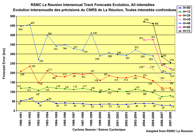
| Season | Analysis | 12 h | 24 h | 36 h | 48 h | 60 h | 72 h |
| 1990 – 1991 (2004 – 2005 for 36, 60 and 72 h) |
52 | 118 | 208 | 235 | 446 | 374 | 470 |
| 2007 – 2008 | 28 | 118 | 120 | 159 | 193 | 221 | 254 |
Table 9.6 shows that for the period 1990-1991 through 2007-2008, model analysis TC location errors reduced from near 50 km to about 30 km and 48 hour track forecast errors were reduced by 60%. Skill varies from season to season, possibly due to seasons in which TC motion was less predictable and/or changes in forecast products or observing systems.
Similar graphical and tabular forecast verifications are compiled for intensity forecasts in each basin. As discussed in Section 9.5.2, intensity forecasts have relatively poor skill, in general, so those forecasts may also be summarized via category. Recently, the NHC began verifying the forecast radii of various wind thresholds by quadrant.
Similar graphical and tabular forecast verifications are compiled for intensity forecasts in each basin. As discussed in Section 9.5.2, intensity forecasts have relatively poor skill, in general, so those forecasts may also be summarized via category. Recently, the NHC began verifying the forecast radii of various wind thresholds by quadrant.
More complex methods of forecast verification are generally reserved for the forecast models. These methods have been evolving quickly. In the last decade or so, model TC forecast verification has expanded beyond track, intensity and rainfall distributions (using spatially distributed, multi-category or entity-based verification methods) to more involved techniques that provide quantitative information on the model skill.
The availability of ensemble forecasts facilitates the need and opportunity for statistically-based verification measures. A few new approaches are discussed next.
http://www.nhc.noaa.gov/verification/verify6.shtml
Example NHC advisories for the 2011 hurricane season
http://www.nhc.noaa.gov/archive/2011/index.shtml
Example Australian BOM TC reports
http://www.bom.gov.au/cyclone/history/index.shtml
9.6 Forecast Verification and Validation »
9.6.2 General Methods for Forecast Verification
Many types of TC forecasts exist, including likelihood of genesis, track and intensity evolution, wind and rain swaths, and watches and warnings; these forecast products are presented in a variety of ways (Table 9.7) and for different domains (Table 9.8). Because of the range of forecast products, each type is evaluated using different verification methods.106,107,108,109 These methods have been developed by international working groups of the WMO World Weather Research Program and World Climate Research Program.110
| Type of forecast | Example forecasts | Verification methods |
| Qualitative (worded)111,112 |
5-day outlook for genesis | visual, dichotomous, multi-category |
| Deterministic (single answer) |
quantitative precipitation forecast | visual, dichotomous, multi-category, continuous, spatial |
| Probabilistic | probability of precipitation, ensemble track forecast | visual, probabilistic, ensemble |
| Space-time domain | Example forecasts | Verification methods |
| Time series | TC storm track or intensity evolution |
visual, dichotomous, multi-category, continuous, spatial |
| Deterministic (single answer) |
TC rainfall chart, wind distribution |
visual, dichotomous, multi-category, continuous, probabilistic, spatial, ensemble |
| Combined space and time | TC rainfall swath, watches and warnings, ensemble tracks | dichotomous, multi-category, continuous, probabilistic, ensemble |
9.6 Forecast Verification and Validation »
9.6.2 General Methods for Forecast Verification »
9.6.2.1 Visual or "Eyeball" Forecast Verification
The quickest way to assess the skill of a forecast in rough terms is to “eyeball” it. One look at the rainfall forecasts below (Fig. 9.79) gives you a sense of the relative skill of the two forecasts for the rainfall distribution of Hurricane Fran (1996). For this case, the GFDL model is more skillful than R-CLIPER.
While visual verification is a great place to start, for a quick reality check, this method is inadequate alone since it is: (i) time consuming, (ii) susceptible to interpretation biases of the observer, and (iii) not a quantitative measure of skill. Without additional quantitative measures of verification, it is hard to determine the relative merits of any forecast procedure over a large set of cases.
9.6 Forecast Verification and Validation »
9.6.2 General Methods for Forecast Verification »
9.6.2.2 Dichotomous (yes/no) Forecast Verification
Dichotomous forecasts provide a clear “yes” or “no” answer to the question “Will this event happen?” Examples of dichotomous forecasts are TC genesis and landfall forecasts. A storm either forms or it does not, it makes landfall or it does not. There are four possible combinations of observations (yes or no) and forecasts (yes or no) for each forecast (Table 9.9). These form the joint distribution of the forecast problem.
| Observed | Forecast | Referred to as |
| Yes, event occurred | Yes, event forecast | Hit |
| No, event not forecast | Miss | |
| No, event did not occur | Yes, event forecast | False alarm |
| No, event not forecast | Correct negative |
The frequency of occurrence of each of these outcomes is easily summarized in a contingency table (Table 9.10), a useful way to see the types of errors being made.
| Frequency of each outcome for a set of dichotomous forecasts | Observed | |||
| Yes | No | Total | ||
| Forecast | Yes | Hits | False alarm | Forecasts to occur |
| No | Miss | Correct negative | Forecast not to occur | |
| Total | Observed | Didn't happen | All cases (same across and down) | |
A perfect forecast system produces only hits and correct negatives, no misses or false alarms.
9.6 Forecast Verification and Validation »
9.6.2 General Methods for Forecast Verification »
9.6.2.3 Multi-category Forecast Verification
Multi-category forecasts are dichotomous forecasts with more than two choices. Instead of a yes/no decision, you decide the category to which each observation and forecast belongs.
Intensity forecasts are examples of multi-category forecasts: the total number of time periods when the set of TCs are (a) tropical storms, (b) hurricanes and (c) major hurricanes can be compared between observations and forecasts. This makes a three-category system, the easiest multi-category system for our example!
Verification of multi-category forecasts starts with a contingency table comparing the frequency of forecasts and observations in the various categories. Examples of multi-category forecasts could include TC category, rainfall intensity ranges (e.g., rainfall rate range by mm day-1), or storm frequency (e.g., active, neutral and inactive season).
Table 9.11 is a multi-category contingency table for a fictional set of TC intensity forecasts. Numbers represent the count of all named storm times for which the intensity category was observed/forecast.
| Evaluation of a Fictional Seasonal Forecast Model | Climatology | ||||
| Major Hurricanes | Hurricanes | Tropical Storms | Total (Forecasts) | ||
| Seasonal Forecast | Major Hurricanes | 180 | 150 | 25 | 355 |
| Hurricanes | 50 | 120 | 90 | 260 | |
| Tropical Storms | 20 | 80 | 285 | 385 | |
| Total (Climatology) | 250 | 350 | 400 | 1000 | |
For a perfect forecast, the only cells containing non-zero values would lie along the diagonal from top left to bottom right. The off-diagonal cells tell us about the specific nature of the forecast errors. The last row and rightmost column of the table show whether the forecast produces the correct distribution of category frequencies. For example, in Table 9.11, major hurricanes are forecasted much more frequently than observed.
The information contained in Table 9.11 is represented graphically in Fig. 9.80. Each set of three bars correspond to the forecast category frequencies that verified as the observed TC category listed along the horizontal axis. For example, the first three bars were all observed to be major hurricanes, but for this set of TC only 180 major hurricanes were forecast, with 50 being forecast only as hurricanes and the remaining 20 as TS.
The advantage of the multi-category approach is that the nature of the forecast errors is more readily diagnosed. The disadvantage is that, by retaining more information, it is harder to condense the results into a single number. However, any multi-category forecast verification can be converted to a series of dichotomous verifications by defining “Yes” to be “in this category” and “No” to be "not in this category.” In our example this could correspond to “Is the (observed/forecast) storm a major hurricane or not?”
9.6 Forecast Verification and Validation »
9.6.2 General Methods for Forecast Verification »
9.6.2.4 Verification of Forecasts of Spatially Distributed Information
Much more information exists in the Hurricane Fran (1996) precipitation forecast example (Fig. 9.79) than we could get from a purely visual inspection, yet by reducing these images to a single number, or even a few numbers, much useful information is lost. While we certainly care about whether or not it will rain, we also care about the rain rate, the area and distribution of heavy rain and its location. Hence, errors in this example might derive from (i) rain rate being too weak or strong, (ii) the rain area being too small or large or incorrectly distributed, or (iii) speed of storm motion. We can reduce the first two questions (whether and how hard) to dichotomous or multi‑category tests but the spatial extent and location of the rain are not so readily reduced.
For our rainfall forecast example, one method of spatial verification is entity-based verification114 (Fig. 9.81). This verification method addresses the questions: “What is the location error of the (spatially distributed) forecast?” and “How does the total error break down into components due to incorrect location, volume, and fine scale structure?”
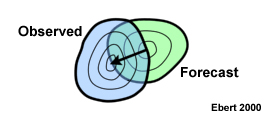
This object-oriented method verifies the properties of spatial forecasts of entities, where an entity is anything that can be defined by a closed contour. Examples of entities are contiguous rain or cloud areas, low pressure centers, and wind maxima. For each entity in the forecast and the observations, object-oriented verification decomposes the total error into the location error, as well as errors in area, mean and maximum intensity, and spatial pattern using pattern matching techniques.
Once observed and forecast entities have been identified, multi-category verification methods can also be applied. For example, each entity can be classified as a “hit", “miss” etc., according to the closeness of the forecast and observed location, and/or the agreement between the observed and forecast maximum intensity.
By invoking multiple thresholds a deterministic forecast system can be evaluated across a range of possible decision thresholds. These might be intensity thresholds or even spatial offsets (e.g., forecast event within 10 km, 20 km, 30 km, etc. of the verifying location). This multi-threshold approach enables a fairer comparison against ensemble prediction systems or other probabilistic forecasts.
Let us return to the Hurricane Fran (1996) precipitation forecast example (Fig. 9.79). Instead of thinking about the rainfall distribution with respect to the storm, we can ask instead, “How much rainfall will State College, PA, receive from Hurricane Fran?” Now we have fixed the location of the rainfall being verified to a point. Note that we still want to know the sources of the forecast error. But now we are interested in how these errors affect a location or region, not the weather system itself. Another method of validating spatially distributed data is to seek the answer to the question,
“What are the spatial scales at which the forecast resembles the observations?”
This can be answered by decomposing a spatially-distributed field (e.g., rainfall, wind speeds) by threshold values, then testing for these threshold values at locations with verifying information. Calculation of a skill score at each location based on the threshold value agreement gives a spatially distributed quantitative measure of skill. A commonly used skill score for spatially distributed forecasts is the Brier Skill Score.b
The most severe test is a point-by-point skill verification, but, if the skill score is calculated over increasingly larger areas, the test is less onerous and the score should improve.
The Fractions Skill Score (FSS)115 an alternative score, is evaluated for areas of increasing size. It ranges between 0 (complete mismatch) and 1 (perfect match). If either there are no events forecast and some occur, or some occur and none are forecast, FSS is always zero.
As the size of the areas used to compute the fractions gets larger, the score will asymptote to a value that depends on the ratio between the forecast and observed frequencies of the event. The closer the asymptotic value is to 1, the smaller the forecast bias. The score is most sensitive to rare events (or for small areas), which may be particularly useful in identifying mismatches between observations and model forecasts of TC wind fields.
b The Brier Skill Score is given as,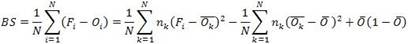 , where the three terms on the right hand side identify errors due to reliability and resolution of the model, and uncertainty of observations respectively. These terms are defined in the discussion of probability forecasts.
9.6 Forecast Verification and Validation »
9.6.2 General Methods for Forecast Verification »
9.6.2.5 Methods for Probabilistic Forecasts
A probabilistic forecast gives a probability, p, of an event occurring, where p is either expressed as a fractional probability (0 ≤ p ≤ 1) or a percentage likelihood (0 ≤ p ≤ 100%).
An accurate probability forecast system has:
- reliability - agreement between forecast probability and mean observed frequency. A model with perfect reliability will always forecast events that occur and have no false alarms;
- resolution - ability of the forecast to resolve the set of sample events into subsets with characteristically different outcomes. Resolution implies that events can be categorized by a multi-category forecast verification of some kind;
- sharpness - tendency to forecast probabilities near 0 or 1, as opposed to values clustered around the mean. If the forecast is always near the mean, we do not have much more information than we could get from climatology.
In addition to the Brier skill score and other similar scores that compare forecast and observed values of chosen variables, another class of skill score is valuable. These are ranked probability scores that provide information on the skill of the forecast in predicting the category that the verifying observation fell into. Example categories you might consider are TC intensities or rain rates.
Ranked Probability Score, RPS
The ranked probability score, RPS, for a set of probabilistic forecasts of category membership is calculated as,
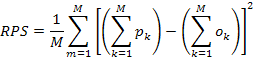 (18)
(18)where M is the number of forecast categories, pk is the predicted probability of an event occurring in category k, and ok is a binary indicator of which category the event occurred in [ok = 0 for false alarm in that category and ok = 1 for correct forecast]. Let us consider an example to illustrate the RPS.
If the forecast probabilities are distributed as follows
Maximum wind
speed category |
Forecast
probability, pk, of intensity in this category |
| 30 - 40 m s-1 | 20% |
| 40 - 50 m s-1 | 50% |
| 50 - 60 m s-1 | 25% |
| 60 - 70 m s-1 | 5% |
| > 70 m s-1 | 0% |
and the observed intensity was 45 m s-1, calculate the RPS using this five category scale.
HINT: Begin by filling in this table
| Maximum wind speed category | Verifying ok | RPSk (contribution to RPS from each category) |
Feedback:
Given an observed intensity of 45 m -1, ok = 1 for the 40 – 50 m s-1 category, and ok = 0 for the remaining four categories. Using this information, we can fill in the table as follows:
| Maximum wind speed category | Verifying ok | RPSk (contribution to RPS from each category) |
| 30 - 40 m s-1 | 0 | 0.04 |
| 40 - 50 m s-1 | 1 | 0.25 |
| 50 - 60 m s-1 | 0 | 0.0625 |
| 60 - 70 m s-1 | 0 | 0.0025 |
| > 70 m s-1 | 0 | 0.0 |
Summing the right hand column gives the answer as RPS = 0.071.
So we see that weighting the probability more strongly in an incorrect category has a large penalty on this score due to the squaring the differences. If the storm had not reached 30 m s-1, the RPS would be exactly one—meaning that the forecast was 100% wrong. If pk = 100% for the 40 – 50 m s-1 category, RPS would have been zero, a perfect forecast of TC intensity in these wind categories.
So, the RPS can be a more reasonable measure of skill, especially in cases such as TC intensity when there is often uncertainty on the actual value, but the likely range of verifying intensity is clear.
Ranked Probability Skill Score (RPSS) measures the relative improvement of the forecast over climatology. One advantage of the RPSS is that it takes the climatological distribution of events between categories into account. Other reference forecasts, such as climatology and persistence, CLIPER, could also be used, but verification of frequencies among categories would then be with respect to these references, not to observed climatology.
Many other measures of the effectiveness of probabilistic forecasts exist. Our discussion is meant to give a flavor of the possible approaches.
9.6 Forecast Verification and Validation »
9.6.2 General Methods for Forecast Verification »
9.6.2.6 Methods for Verification of Ensemble Forecasts
As we discussed in Section 9.4.5Section 9.4.5, ensembles consist of many versions of a single dynamical model or many different dynamical models. The ensemble forecast captures the uncertainty in the forecast and provides a range of outcomes.
Many methods for evaluating probability forecasts can also be implemented for evaluating ensemble forecasts, where the spread of the ensemble members indicates probability. However, since ensembles provide information on the range of possible outcomes given the particular initial conditions, other measures of skill can also be applied to ensembles. We review just a few. You are encouraged to explore further using the cited references and resource links.
- Rank histogram The rank histogram is a quantitative, multi-category method of verification that is represented visually (e.g., Fig. 9.82). It measures how well the ensemble spread of the forecast represents the true variability (uncertainty) of the observations. It is also known as a “Talagrand diagram”.116,117
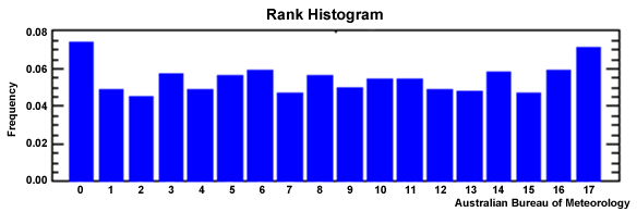
In an ensemble with perfect spread, an observation is equally likely to fall between any pair of ensemble members since each ensemble member represents an equally likely scenario. Therefore, we can evaluate the success of the ensemble spread by looking at the shape of the rank histogram. If the histogram is:
- Flat, the ensemble spread is acceptable for representing the forecast uncertainty. Note that a flat rank histogram does not necessarily indicate a good forecast, only that the ensemble is a reasonable representation of the observed probability distribution;
- U-shaped, the ensemble spread is too small since many observations fall outside the range spanned by all of the ensemble members.
- Dome-shaped, the ensemble spread is too large since most observations fall near the center of the range of the ensemble set;
- Asymmetric, the ensemble has an overall bias compared to observations.
Verifying forecasts of rare and/or extreme events
Since we are interested in verification for ensemble forecasts of TC, we will briefly review two methods for verifying ensemble forecasts of rare and extreme events.
- Deterministic limit
The deterministic limit118 is the forecast lead time at which the number of misses plus false alarms in the ensemble forecast set equals the number of hits for a chosen weather system. It measures the forecast lead time for which the forecast is more likely to be correct than incorrect (Fig. 9.83). While this may not sound too exciting, it could help the forecaster to decide how much weight to give that forecast and, possibly, to decide to switch from deterministic to probabilistic guidance.
One example of the use of a deterministic limit would be the statement that “The deterministic limit for forecasts of TC intensity by the XXX model is 24 hours.”
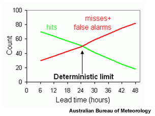
- Extreme Dependency Score
The Extreme Dependency Score (EDS) measures the reliability of a model to forecast a specific weather system, such as a TC. The EDS119 is a measure of the forecast skill for observed rare events. It ranges between -1 and 1, where a perfect score is EDS=1.
http://www.dtcenter.org/met/users/index.php
Survey of common meteorology model verification methods,
http://cawcr.gov.au/bmrc/wefor/staff/eee/verif/Stanski_et_al/Stanski_et_al.html
Forecast accuracy and verification scores,
http://www.eumetcal.org.uk/euromet/courses/english/navig/beginn.htm
Statistical challenges for verification of forecasts of weather extremes,
http://cawcr.gov.au/bmrc/wefor/staff/eee/verif/Casati/statxtr.htm
How do I know whether one model is better than another?
http://cawcr.gov.au/bmrc/wefor/staff/eee/verif/CIdiff/FAQ-CIdiff.html
9.6 Forecast Verification and Validation »
9.6.3 Summary: Advantages and Inadequacies of Current TC Forecast Models
Based on results from the current verification methods, we can make some general comments on the skill of the current generation of forecast models.
While it is possible for the human forecaster to show skill over the operational forecast models from time to time, model performance has improved significantly over the years, and they are now very difficult to beat on a consistent basis, at least for track forecasts.
Intensity forecasting is much more complex than track forecasting. For a start, intensity forecasts rely in some measure on the track forecasts (e.g., to get interactions with other weather systems and SST information). Further, intensity depends on details of the TC core structure, such as the distribution of deep convection, and other internal storm processes. Thus, dynamical forecast models still have little skill in predicting TC intensity change.
Statistical models for TC intensity are beginning to provide useful guidance, although since they are built using historical storm information, their skill is restricted to “typical” TC intensity evolution. Events such as rapid intensity change are not well forecast in either statistical or dynamical models. Current statistical models of rapid intensity change are based on a very small set of storms, which limits the range of possible intensity changes that underlie the statistical model.
Consensus forecast systems offer hope for improvements in forecast accuracy. Ensemble prediction systems are beginning to address the problem of TC forecasting directly101,120 by targeting TC when the ensemble perturbations are developed,80 rather than developing the perturbations as part of a larger forecasting problem. These offer hope of improved forecasts, not only of TC track and intensity, but on wind and rainfall distributions and storm structure evolution. Forecasting of extratropically transitioning TC121 (ET, Section 8.5ET, Section 8.5) and the influence of these ET systems on the midlatitude flow122,123 is also a critical problem being studied using these targeted model ensembles.
Focus Areas
Focus Areas »
Focus 1: The Australian-Indonesian Monsoon
Focus 1: The Australian-Indonesian Monsoon »
9F1.1 Overview of the North Australian Monsoon
by Dr. Mick Pope of the Australian Bureau of Meteorology (BoM)
The monsoon refers to the tropical and subtropical seasonal reversals in the atmospheric circulation and associated precipitation,124 leading to two distinct phases, “wet” and “dry” (Fig. 9F1.1).125 The changes in the atmospheric circulations arise from reversals in temperature gradients between continental regions and the adjacent oceans. In many cases this is accompanied by the seasonal migration of the Hadley cell and associated monsoon trough or ITCZ. However, in the case of the American monsoons (Fig.9F1.1, left panels), no seasonal reversal of the winds has been identified.125 Equatorial regions have two rainy seasons and the trade wind flow collects moisture over the warm tropical oceans. In locations like Australia and India, one rainy season occurs when the cross equatorial flow turns westerly (Fig. 9F1.1, right panels). The corresponding trade wind easterlies are dry and characterized by a low-level inversion which caps deep convection.
This focus section will examine the Australian-Indonesian monsoon as a case study of monsoon dynamics, with a particular focus on the differences between the various intraseasonal phases.
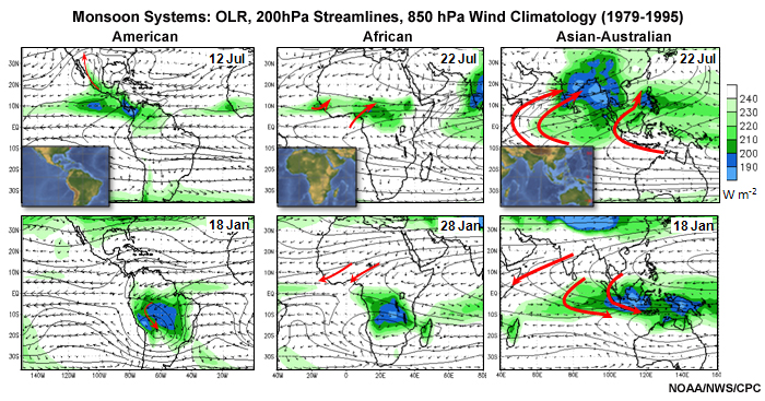
Focus 1: The Australian-Indonesian Monsoon »
9F1.1 Overview of the North Australian Monsoon »
9F1.1.1 The Seasonal Cycle
Like the Indian monsoon,126 the Australian-Indonesian monsoon undergoes intraseasonal variation consisting of active and break phases, characterized by widespread and isolated precipitation respectively (Fig.9F1.2).
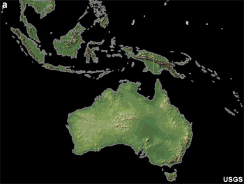
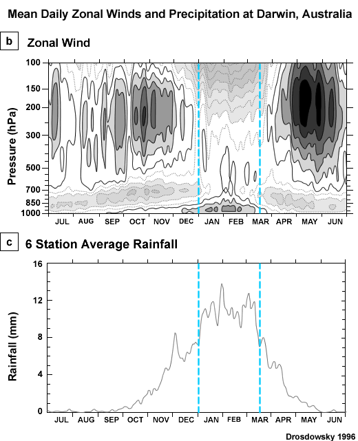
The NAM forms part of the global monsoon driven by the Hadley Cell. Up motion occurs in the hot towers due to condensational heating, resulting in lower pressures near the surface in the tropics and hence a cross equatorial pressure gradient with the winter hemisphere mid-latitudes. The column heating in the hot tower also produces a much stronger reverse pressure gradient in the upper troposphere which drives the upper return flow into the winter hemisphere.127 Modeling studies show that the response to the tropospheric heating is stronger when the heating is off the equator.128 Superimposed on this is the land-sea thermal contrast that develops during Austral Spring.125 A heat low develops over the Pilbara region, often resulting in shallow westerly flow over northern Australia, which moistens and pre-conditions the environment for deep convection (Fig.9F1.3). The period during which this pre-conditioning and isolated shallow convection occurs is known as the buildup. There is also a forcing due to the seasonal migration of the warmest sea surface temperatures.129
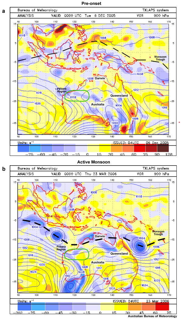
![]() A significant amount of rainfall occurs outside of the period of westerly winds. What weather systems would be responsible for this? We will answer this question in a later section.
A significant amount of rainfall occurs outside of the period of westerly winds. What weather systems would be responsible for this? We will answer this question in a later section.
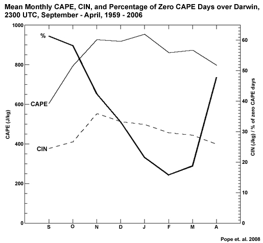
The seasonal cycle can also be considered in terms of the CAPE—a proxy for the strength of convective updrafts. The most energetic updrafts occur on average during November to January. Figure 9F1.4 shows the month values of CAPE, Convective Inhibition (CIN) and number of zero CAPE days for the 2300 UTC Darwin sounding. The amount of CAPE almost doubles during the late dry season (September through November), with a rapid decrease in the number of zero CAPE days. The increase in the CIN during this period is likely an artifact of the large number of zero CAPE days during September and October. Zero CAPE days reach a minimum at the peak of the monsoon during February, although this is not the time of maximum mean monthly CAPE.
Focus 1: The Australian-Indonesian Monsoon »
9F1.2 Regimes of the North Australian Monsoon
Focus 1: The Australian-Indonesian Monsoon »
9F1.2 Regimes of the North Australian Monsoon »
9F1.2.1 TWP-ICE
The NAM undergoes significant intraseasonal variability. Figure 9F1.5 shows the area average rain accumulation for January and February 2006 from the Tropical Warm Pool – International Cloud Experiment (TWP-ICE).131 The active period of the monsoon was marked by deep zonal westerly winds over Darwin and, during 23-26 January, an intense mesoscale convective system (MCS) produced an area averaged rainfall rate of approximately 45 mm day-1. The period starting February 6th is referred to as a break monsoon with deep tropospheric easterly winds, which produced an area averaged rainfall rate of approximately 8 mm day-1.
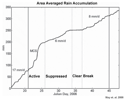
The NAM is characterized by active and break periods.132,133,134 During periods when the MJO is active (which it is not during all summers) there is a strong synchronization between the active-break cycle and the MJO.135,136 Likewise, the greatest probabilities of rainfall in the highest quintile are observed during the active MJO phase. Other influences on the monsoon at Darwin include upper troughs137 and equatorially-trapped Rossby wavesequatorially-trapped Rossby waves.138
The unusual phenomenon observed during TWP-ICE was the suppressed period of relatively small rainfall, together with the three days of clear conditions over Darwin with no rainfall. We now consider these three monsoon regimes in more detail.
Focus 1: The Australian-Indonesian Monsoon »
9F1.2 Regimes of the North Australian Monsoon »
9F1.2.2 The active monsoon
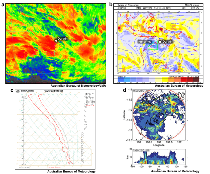
The active monsoon is associated with widespread, deep tropical convection, indicated by cold clouds in the IR image (Fig. 9F1.6a); although some cold clouds may be cirrus as IR cannot distinguish between precipitating convection and cold cirrus (Chapter 2, Section 2.5.2Chapter 2, Section 2.5.2). The associated synoptic pattern is a deep low over the Kimberley, directing west to northwesterly winds over northwest Australia and surrounding waters. The Monsoon Trough (MT) is indicated by the east-west oriented cyclonic vorticity maximum. Equatorward of the MT, the flow is converging into the low, resulting in the observed cloudiness and vertical motion profile (Fig. 9F1.6a,c). The sounding shows a typical active monsoon profile with a small dewpoint depression through the depth of the troposphere and a lapse rate close to moist adiabatic. The CAPE is typically small during the active monsoon. The wind profile is westerly to approximately 400 hPa with easterly winds above that. Drosdowsky (1984)139 defined the active monsoon in terms of the wind profile, with mean westerly zonal winds to 500 hPa and mean easterly zonal winds above 300 hPa.
Which weather elements are likely to be important in an active monsoon environment? What timing for the onset and cessation of these events might be appropriate and why? (Type your answer in box.)
Feedback:
Below is an example of the evolution of convective weather expected during an active monsoon; as expressed in a Terminal Aerodrome Forecast (TAF).
TAF YPDN 171802Z 1718/1818 34015KT 9999 SCT020
TEMPO 1718/1802 30020G40KT 1000 TSRA BKN010 SCT020CB
INTER 1802/1810 30020G40KT 3000 +SHRA BKN010
TEMPO 1810/1818 31020G40KT 1000 TSRA BKN010 SCT020CB
The Terminal Aerodrome Forecast (TAF) for Darwin shows periods of reduced visibility, lowered cloud base and precipitation in the form of heavy rain showers (+SHRA) and thunderstorms with rain (TSRA) throughout the validity period of the forecast which is 24 hours from 1800 UTC (0330 LST). An INTER means that conditions persist for periods of 30 minutes or less, a TEMPO for periods between 30 minutes and 1 hour.
During the thunderstorms described by the TAF above, the visibility is down to 1 km and in heavy showers to 3 km. The term BKN010 refers to low cloud with a base of 1000 feet, covering between 5 and 7 oktas (eighths) of the sky. The 24-hour coverage is consistent with the widespread cloud cover observed and the presence of synoptic-scale convergence and upward motion (Fig. 11F1.6). The focus of deep convection during the night and morning hours (between 1000 UTC = 1930 LST and 0200 UTC = 1130 LST) implies that deep convection is more likely to be nocturnal during the active monsoon, characterizing the airmass as maritime. The use of the TEMPO for this length of time is designed to include the time of potential enhanced convection and associated reduced visibility and cloud base due to the convection and enhanced by the wet bulb process. The peak in number and strength of updrafts does not typically occur until after dawn (about 0700 0900 LST).
Focus 1: The Australian-Indonesian Monsoon »
9F1.2 Regimes of the North Australian Monsoon »
9F1.2.3 The Break Monsoon
In contrast to the active monsoon, clouds are more isolated during the break periods (Fig. 9F1.7), often coastal, due to triggering on the sea breeze, and westward propagating. The MSLP/vorticity plot shows that the MT is to the north of Darwin, extending from the Arafura Sea into the Coral Sea. A region of cyclonic vorticity lies along the west coast of Australia extending into a heat low.
What differences do you observe between the trace (sounding) for the break monsoon period (shown below in 9F1.7c) ) and the active monsoon? (Type your answer in box.)
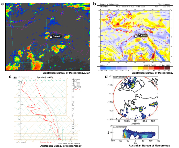
Feedback:
The main features of the sounding are easterlies through most of the troposphere compared to the westerlies of the active monsoon. The shallow westerlies near the surface are a result of the heat low. The zig-zag pattern in the dewpoint profile indicate dry air in mid-levels, referred to as dry slots.
Where on the satellite image, in Fig. 9F1.7, do you expect the sea-breeze front to be found over northern Australia? (Type your answer in box.)
Feedback:
Where on the satellite image do you expect the sea-breeze front to be found?
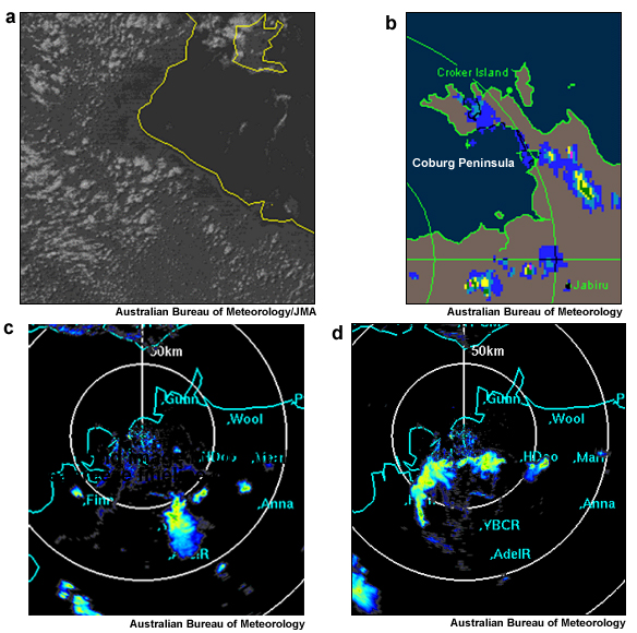
Convection usually occurs at the leading edge of the sea-breeze front,140 where the warm and moist inland air of the prevailing flow is lifted to its level of free convection. The orientation of the prevailing flow determines the preferred locations of convective development (Fig. 9F1.8). Convective rolls are also generated inland. The air mass coastward of the sea-breeze front is indicated by the cloud free region along the coast. On the radar image, the sea-breeze front is indicated by the line of convection parallel to the coast. Convection along the Coburg peninsula is indicative of the convergence of sea breezes (Fig. 9F1.8b).
The sea-breeze front also interacts with existing convection. In Fig. 9F1.8c, the sea-breeze front is seen as a light blue line oriented from Humpty Doo (HDoo) to Finnis Range (Finn). A thunderstorm propagates in from the southeast. Once the storm reaches the sea-breeze front, the outflow interacts with the sea breeze to initiate fresh convection, in this case, a squall line propagating to the northwest.
Compare the Darwin TAF for the break period (below) with the one for the active periodactive period. What differences do you observed for the wind? How does this relate to the differences in synoptic regime? What differences are observed in the key weather elements and timing?
TAF YPDN 061611Z 0618/1818 22007KT 9999 SCT020 FM0802 30014KT 9999 SCT030
TEMPO 0706/0612 10015G35KT 1000 TSRA BKN010 SCT020CB
(Type your answer in box.)
Feedback:
The winds are northwesterly in the active monsoon but here the wind is southwesterly turning northwest during the morning. Thunderstorms are forecast during the afternoon and evening, compared to showers and storms for the active monsoon. The TEMPO is diurnal rather than through the period, indicating that the trigger convection is due to the sea breeze and surface heating.
Focus 1: The Australian-Indonesian Monsoon »
9F1.2 Regimes of the North Australian Monsoon »
9F1.2.4 Comparison Between the Active and Break Periods
Given the mean diurnal cycle for the Australian-Indonesian monsoon shown in Section 5.3.7.2Section 5.3.7.2, what differences would you expect between the active and break periods for a place like Darwin?
(Type your answer in box.)
Feedback:
The active and break monsoon environments have different synoptic forcing and air masses. These differences should be reflected in the diurnal cycle of the resulting deep convection, as has been suggested by the TAFs of the activeactive and break break periods shown earlier. Figures 9F1.9 and 9F1.10 compare the diurnal cycles of convection for different phases of the monsoon.
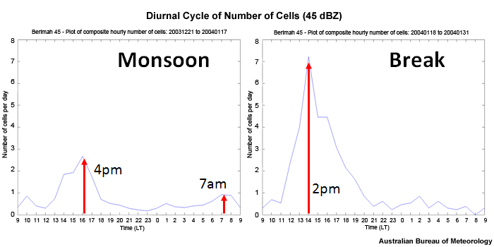
The break period has a strong diurnal signal, with a peak at 1400 LST. The timing of this peak is location dependent. It depends on the day to day synoptic forcing, sea-breeze cycle, and occurrence of earlier convection which may suppress the environment. The active period has a relatively flat diurnal cycle, with a weaker diurnal maximum at 1600 LST, compared to the break, and a morning peak at 0700 LST. The relatively flat diurnal cycle is consistent with the maritime nature of the air mass.
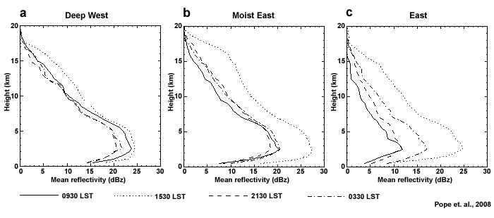
Another way to illustrate the diurnal cycle is to compare the mean reflectivity versus height (Fig. 9F1.10). The active monsoon has a very weak diurnal cycle with maximum values at 0930 and 1530 LST. The break period has a flat diurnal cycle except for the pronounced afternoon peak at 1530 LST when the mean reflectivity increases by 10 dBZ over most of the depth of the troposphere. The buildup profile is typical of the early wet season, when the surface moisture is still increasing. The echoes are not as deep as the break period or as large for a given height, indicating weaker updrafts. This is due to the entrainment of drier environmental air in the boundary layer. The gradual increase in reflectivity during the diurnal cycle is consistent with the mechanism by which multiple plumes moisten the atmosphere and allow larger rain droplets to form.
![]() What differences will the amount of convection make to the thermodynamics of the active and break regions and vice versa?
What differences will the amount of convection make to the thermodynamics of the active and break regions and vice versa?
Active or break environments occur relative to the monsoon trough, as shown in Fig. 9F1.11. In the southeasterly stream poleward of the monsoon trough at O, dry air advection results in the dry slots observed in the dewpoint profile. Equatorward of the monsoon trough at X, moist maritime air is lifted in the convergent region to produce a deep moist profile. The animation of Fig. 9F1.11 illustrates that, as the monsoon trough migrates poleward, winds shift from easterly to northeasterly with southeasterly flow in the upper troposphere to deep monsoon westerly with easterly flow aloft. Tropospheric moisture increases with the change in trajectories and synoptic forcing.
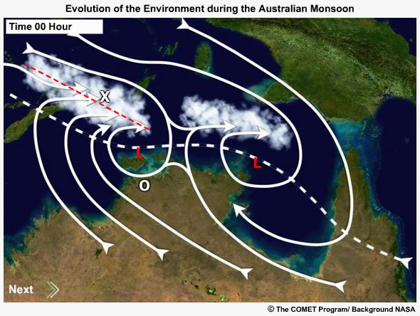
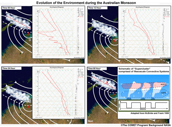
The cross section (shown by rolling over X in animation of Fig. 9F1.11) illustrates the difference in CAPE and lapse rate between the active and break period environments. Latent heat release in the mid to upper troposphere warms the environment while evaporation of precipitation cools the lower troposphere, stabilizing the lapse rate. Spreading near surface cold pools reduce the CAPE by bringing down cooler and drier air from aloft. During break periods, shortwave heating of the surface and longwave cooling of the atmosphere destabilize the troposphere and allow CAPE to recover.
Focus 1: The Australian-Indonesian Monsoon »
9F1.2 Regimes of the North Australian Monsoon »
9F1.2.5 The Suppressed Monsoon
Refer back to Fig 9F1.5. What kind of synoptic environment could produce a suppressed regime?
(Type your answer in box.)
Feedback:
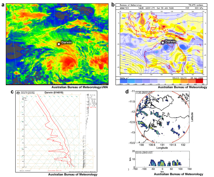
The suppressed monsoon over Darwin is due to a deep low over central Australia (Fig. 9F1.12). Such deep lows are referred to colloquially as ‘landfoons’ due to their structural similarity to tropical cyclones (also known as typhoons) in the satellite imagery and their potential to become tropical cyclones were they over the warm, tropical ocean.143 The MSLP/vorticity chart shows that the monsoon trough is well to the south of Darwin, together with the associated convergence. The flow is southwesterly rather than the west to northwesterly flow associated with an active monsoon.
Compare the trace (sounding) of the suppressed monsoon to the trace for the active monsoon. How is the wind profile similar/different? How is the dewpoint profile different?
(Type your answer in box.)
Feedback:
The winds are strong westerly as is the case for the active monsoon, but the meridional component is southerly. The ‘dry slots’ in the dewpoint profile look like those in the break period monsoon profile. The suggestion is that the trajectories are different due to the location of the low; advecting drier air from further south. Examination of model moisture fields and backward trajectories confirms this.
What differences will the drier trajectories produce in the Darwin? Is deep convection likely?
(Type your answer in box.)
Feedback:
Below is a description of the weather situation including an example TAF.
TAF YPDN 271613Z 2718/2818 27020G30KT 9999 BKN020
INTER 2718/2818 26020G40KT 4000 SHRA BKN010
The TAF indicates an INTER (less than 30 minutes at a time) showers only which indicates a relatively suppressed environment, i.e., no deep convection. Note that Fig. 9F1.5 indicates that, as the low moved further south, conditions became more suppressed so that eventually no showers were observed.
The occurrence of the suppressed monsoon highlights the shortcomings of zonal wind only based definitions of monsoon onset. More work is required to more rigorously define the regimes of the NAM.141
Focus 1: The Australian-Indonesian Monsoon »
9F1.2 Regimes of the North Australian Monsoon »
9F1.2.6 Summary of NAM Regime Differences
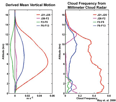
The active monsoon is dominated by deep upward motion, reaching a maximum near 6 km, and a large cloud frequency (red line in Fig. 9F1.13). Although the break monsoon period contains some intense storms, their isolated nature and differences in the large scale forcing means that the mean vertical motion is much less than the active monsoon (blue line in Fig. 9F1.13). The suppressed monsoon has very weak mean vertical motion, and the vertical cloud frequency profile shows the prevalence of shallow convective cloud mostly below 3 km, together with the cirrus between about 10 and 14 km. The cloud free period is unsurprisingly associated largely with subsidence.
Focus 1: The Australian-Indonesian Monsoon »
9F1.3 Storm Types of the North Australian Monsoon
This section examines some of the convective weather systems associated with the NAM. It is not an exhaustive treatment.
Focus 1: The Australian-Indonesian Monsoon »
9F1.3 Storm Types of the North Australian Monsoon »
9F1.3.1 Wet Microbursts
A wet microburst is a thunderstorm which produces damaging surface winds associated with significant precipitation at the surface and a low cloud base (Fig 9F1.14). Typically, the moisture extends to about 500 hPa with a dry layer above and the wind shear is weak. The low cloud base is due to high relative humidity near the surface, inhibiting evaporation. A warm cloud depth of greater than 10000 ft allows the collision and coalescence process to produce large rain drops. These conditions imply that precipitation drag is important in forming the downdraft. These storms occur during active and break monsoon conditions.
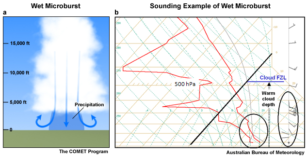
On 31 January 2000 wind gusts of 100 and 150 km h-1 were produced by a sustained wet microburst of about 30 minutes in duration. Figure 9F1.15 shows the Doppler velocities for a wet microburst. Figure 9F1.15 also shows the effect of large CAPE on a wet microburst environment. Large CAPE result in strong updrafts which produce elevated strong reflectivity echoes, making it possible to detect an impending downburst before it occurs. For small to moderate CAPE (< 2000 J kg-1) the first echoes are observed at about 3–6 km (10–19000 ft). These typically produce non-severe wind gusts. For larger CAPE, first echoes are observed at about 7–9 km (22000–30000 ft).
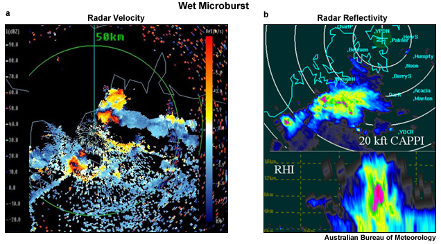
Focus 1: The Australian-Indonesian Monsoon »
9F1.3 Storm Types of the North Australian Monsoon »
9F1.3.2 Dry Microbursts
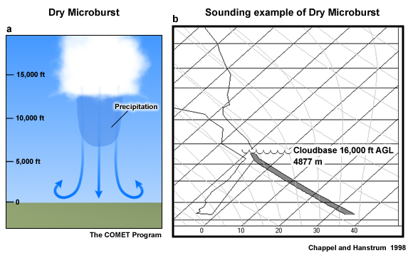
Dry microbursts are a feature of inland Australia in an environment of deep easterly flow where the boundary layer is deep (up to 16000 ft above ground level) and dry. These storms produce damaging winds at the surface with no precipitation. Updrafts are weak due to low CAPE and vertical wind shear is weak. Hence, the downburst is produced by evaporation. The trace shown in Figure 9F1.16 was observed at Alice Springs aerodrome in 1992, and produced wind gusts of 72 and 94 km h-1. These storms are difficult to forecast because mixing with the hot environmental air and weakens the negative buoyancy of the downdraft. These storms occur during active and break monsoon conditions.
Focus 1: The Australian-Indonesian Monsoon »
9F1.3 Storm Types of the North Australian Monsoon »
9F1.3.3 Continental Squall Lines
Continental squall lines occur during break phases of the monsoon and can produce potentially damaging surface winds. A typical continental squall line, approaching Darwin from the east, consists of a leading edge of deep convection with a trailing stratiform region (Fig. 9F1.17).
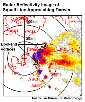
The basic conceptual model of a squall line is a line of convection propagating perpendicular to the mean wind shear vector or mean steering flow (COMET’s Convective Matrix). The strong unidirectional wind flow provides wind shear to balance the vorticity generated at the leading edge of the spreading cold pool by buoyancy gradients to generating new convective cells at the leading edge (Fig. 9F1.18). The wind profile also provides winds to ingest in the convective downdraft as surface gusts. The cold pool is produced by the evaporation of precipitation falling through unsaturated environmental air, known as the dry slot.
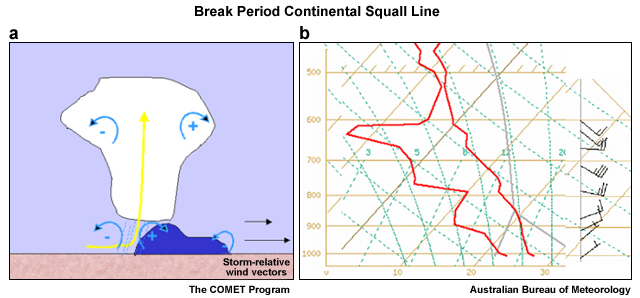
One of the signatures of a severe squall line is the rear inflow jet. Strong rear inflow jets occur in large CAPE, strong vertical wind shear environments. The rear inflow jet accelerates the flow into the rear of the squall line and hence increases the potential surface wind gusts.
Eventually, the cold pool outruns its parent convection and the squall dies. At this stage, the strongest surface winds occur as the rear inflow jet reaches the surface in the downdraft (Fig. 9F1.19). Evidence of a rear inflow jet and imminent surface wind gusts can be obtained from Doppler radar. Fig. 9F1.19 shows Doppler imagery with double range folding to 25 m s-1 (~ 50 kts) 9 minutes before the measured gust of 58 knots at the surface. A thin region of dark blue indicates this range folding, moving through orange shades and then through again to dark blue "circular" regions.
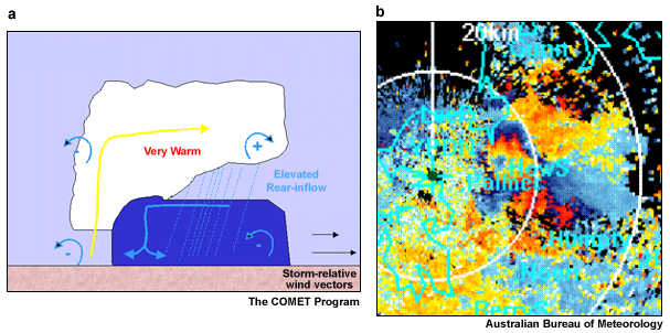
Another feature of potential severity for squall lines is the bookend vortex. Bookend vortices result from vorticity at the leading edge of the cold pool being lifted and tilted by the updraft (reference). The bookend vortices can increase the strength of the rear inflow jet and cause part of the squall line to bow outwards as a bow echo. Figure 9F1.17 shows a bow echo, as well as curved elements in the reflectivity at either end of the leading edge, indicative of bookend vortices.
Focus 1: The Australian-Indonesian Monsoon »
9F1.3 Storm Types of the North Australian Monsoon »
9F1.3.4 Monsoon Squalls
A monsoon squall, also referred to as maritime squalls, form in an environment of deep westerly winds. The lines occur in regions of moderate to strong wind shear in the lower troposphere, and with a block of strong westerly winds. Figure 9F1.20 shows an example of a series of linear features with strong surface winds moving over the Tiwi Islands. A large dry slot exists between 800 and 500 hPa. One monsoon squall on 3 January 2005 produced several convective lines resulting in gusts observed up to 110 km h-1.
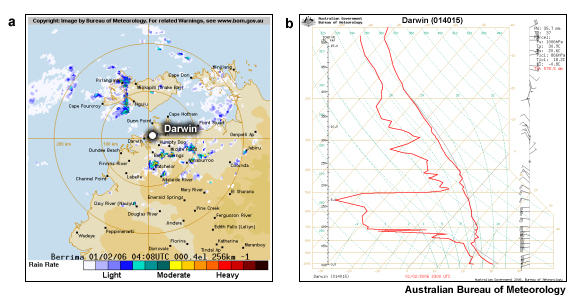
Focus 1: The Australian-Indonesian Monsoon »
9F1.4 The Monsoon over the Maritime Continent
Focus 1: The Australian-Indonesian Monsoon »
9F1.4 The Monsoon over the Maritime Continent »
9F1.4.1 Hector and Convection over Flat Islands
Hector is a thunderstorm complex occurring over the Tiwi Islands, with a height > 15 km, and a horizontal extent of the > 30 dBZ echo of at least 200 km2.145 Hector forms during the break periods of the monsoon. The zonal tropospheric wind flow during this period is easterly, providing the steering flow as is the case for tropical squall lines. The direction of the low-level flow determines where convective initiation starts (Fig. 9F1.21). Figure 9F1.21 also shows the evolution of Hector when the low-level flow is westerly, such as occurs when there is an active heat low over mainland Australia. Convection is preferentially initiated on the eastern side of the Tiwis on the sea-breeze front (Fig. 9F1.21). Weaker convection is initiated on the western coast on a weak sea-breeze front. As the initial convection evolves from updraft dominated (a) to downdraft dominated (b), the spreading cold pool becomes the new site of convective initiation as the cold pool vorticity balances the wind shear. Further lifting occurs as Hector propagates westward and the cold pool interacts with the western sea-breeze front. A radar sequence of a developing Hector is shown in Fig. 9F1.22.
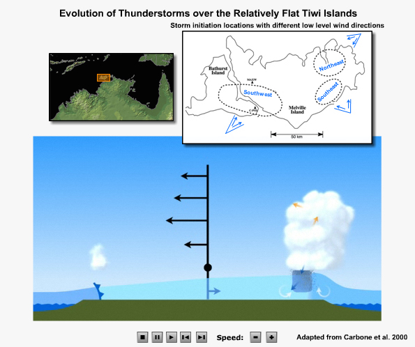
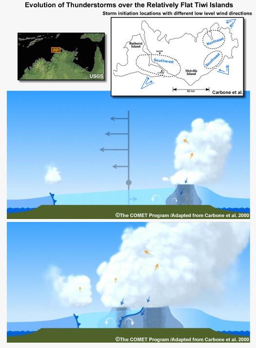
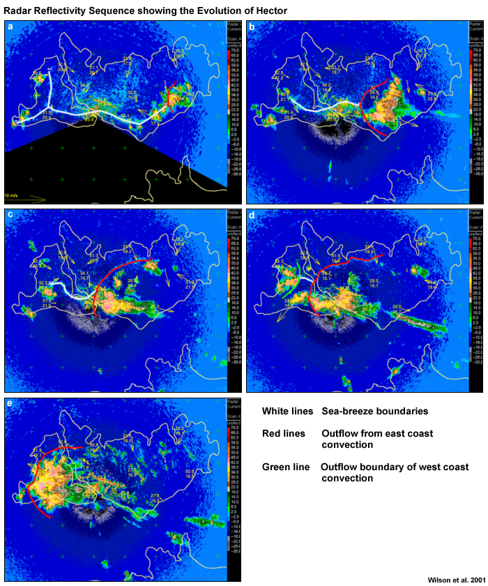
The key element of Hector is that it occurs on an island with little rugged topography, allowing the entire mesoscale convective system to propagate across the island. The site of initial convective initiation is determined by the low-level flow, and thereafter Hector propagates to the west.
What do you think happens in the case of islands with significant rugged topography?
(Type your answer in box.)
Feedback:
We will explore those situations in the following section.
Focus 1: The Australian-Indonesian Monsoon »
9F1.4 The Monsoon over the Maritime Continent »
9F1.4.2 Timor and Convection over Significant Topography
Timor is an island with significant mountains. The highest point reaches 2963 m (9721 ft). Figure 9F1.23 shows the situation for two days in February 2006 with similar gradient level wind flow (3000’ above sea level). However differences in the wind profiles give rise to differences in convective cloud initiation and evolution (compare the left and right panels of Fig. 9F1.23). On the 8th the flow is east to northeast whereas on the 10th (11th was unavailable) flow is weak for much of the depth of the troposphere. On the 8th, the convection appears to form further inland along the spine of the island and is steered along the ranges. Later on the 8th, shallower convection in the Timor Sea is steered towards the northeast by the lower tropospheric flow. The slightly weaker near surface flow on the 11th allows convection to be generated near the coast, and on the ranges to the West of Dili. The steering flow then carries this convection into the Savu Sea.
What impact will these different situations have on forecasting for Dili airport? Review Fig. 9F1.23 before making your forecast.
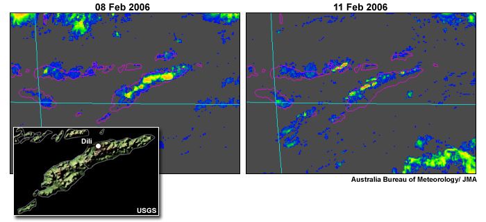
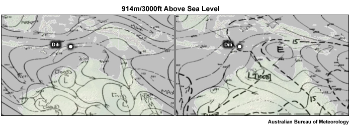
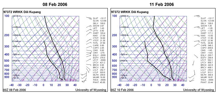
(Type your answer in box.)
Feedback:
An expert response:
TAF WPDL 080105Z 0801/0814 31008KT 9999 BKN025
FM0813 14003KT 9999 SCT020
PROB30 INTER 0805/0810 5000 SHRA BKN010
TAF WPDL 110107Z 1101/1114 29011KT 9999 SCT025
PROB30 TEMPO1105/1111 1000 TSRA BKN010 SCT020CB
A chance of thunderstorms and rain (30% probability) at Dili was forecast on the 11th as the steering flow was easterly, possibly advecting the storms off the ranges and over Dili. On the 8th the steering was along the ranges so only showers and fewer clouds were forecast at Dili.
Focus 1: The Australian-Indonesian Monsoon »
9F1.4 The Monsoon over the Maritime Continent »
9F1.4.3 Papua New Guinea
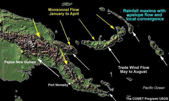
Papua New Guinea’s (PNG) climate may not be described as truly monsoonal as there are no reliable periods of nil or near nil monthly rainfall as there is in Darwin, for example. Rainfall on the highlands is in the range 2500-3500 mm, with somewhat lesser values in the lowland areas. For example, Port Moresby has less than 1000 mm per year. Despite being tropical, frosts can occur above 2200 m and snow settles above 4000 m.
PNG rainfall is enhanced over the tropical oceanic regions due to two factors:
- the mountains of the Maritime Continent
- the West Pacific warm pool
Both contribute to the maintenance of high θe air in this area. From routine satellite imagery, it can be seen that, cloud associated with the ITCZ affects PNG all year. However, the associated wind circulation patterns and the nature of the weather disturbances vary seasonally (Fig. 9.24).
During the southeasterly trades, convergence occurs where flow is onshore and undergoing frictional convergence and collision with nighttime land breezes (Fig. 9F1.24). During the monsoon, these convergences occur in different locations (Fig. 9F1.24). Throughout the year, enhanced uplift due to local topography leads to convection.146 Mountain-valley circulations also contribute to local convergence and convection.
Focus 1: The Australian-Indonesian Monsoon »
9F1.4 The Monsoon over the Maritime Continent »
9F1.4.4 The Indonesian-Malaysian Region
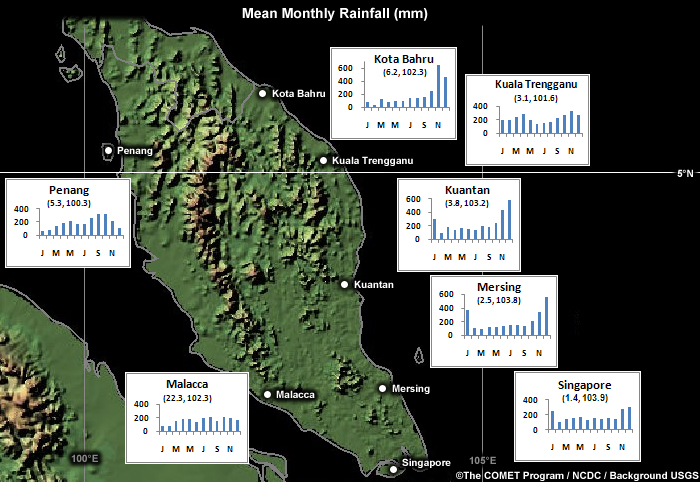
As was the case for PNG, enhanced topography can play a key role in the seasonal variation of rainfall throughout the Maritime Continent.147 Close to the equator there is a much less marked difference between wet and dry seasons than for the NAM. For example, Singapore has a relatively flat rainfall distribution (Fig. 9F1.25). The local rainfall minima occur in July and February under the influence of dry trade wind flows. The further north along the east coast, the greater the topographical enhancement of rainfall during the Boreal Winter (northeast) Monsoon. For example, the November rainfall at Kota Bahru is twice that of Singapore. Likewise, on the northwest coast a secondary peak exists in rainfall during April-May due to the southwesterly cross equatorial flow and the elevated topography.
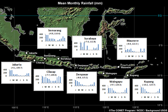
Java has a distinct dry season (Fig. 9F1.26), particularly in the south when under influence of southeast trade winds in the southern hemisphere (May to September). Likewise, there is a distinct wet season when influenced by Boreal Winter Monsoon (northeast trade winds). Sumatra (Fig. 9F1.27) also has a dry season under the influence of the southern hemisphere trades (May to September). The wet season is bimodal where mountains are able to enhance the northeast and southwest flows during boreal winter and summer respectively.
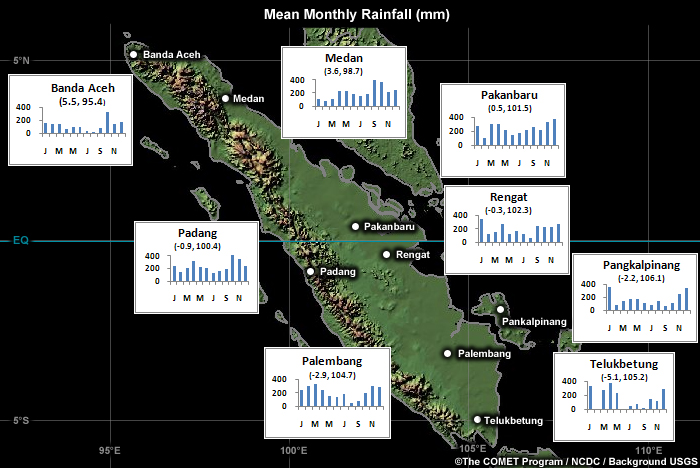
Intraseasonal variability
As with northern Australia, the MJO and various tropical wave modes such as the Kelvin wave, n=1 equatorial Rossby wave and mixed Rossby-gravity wave are responsible for intraseasonal variability over the Maritime Continent (Chapter 4, Section 4.1Chapter 4, Section 4.1) and references therein). Real-time monitoring of the MJO (Table 4.1)Real-time monitoring of the MJO (Table 4.1) and various tropical wave modes (Table 4.2various tropical wave modes (Table 4.2) is done routinely by NOAA and the Australian BoM.
However, as illustrated earlier in this section, knowledge of local topography is essential for forecasting rainfall over the Maritime Continent. For example, Haylock and McBride (2001)148 showed that the coherence of rainfall anomalies during December to February for two rainfall stations on Java separated by less than 100 km was small (correlation of 0.18).
NOAA/ESRL/PSD, OLR Modes, http://www.esrl.noaa.gov/psd/map/clim/olr_modes/
Australian BOM, Real-time and Forecasted Tropical OLR Modes,
http://cawcr.gov.au/staff/mwheeler/maproom/OLR_modes/
Focus 1: The Australian-Indonesian Monsoon »
9F1.5 Summary of the North Australian Monsoon
The differences between active, break and suppressed monsoon regimes for the North Australian Monsoon (NAM) are summarized in Fig. 9F1.28. The NAM is a result of the annual land-sea thermal contrast that develops during Austral Spring superimposed on the seasonal migration of the Hadley cell. The NAM is modulated by the Madden Julian Oscillation, upper troughs and equatorial waves, as well as by an inherent transient component of monsoon systems.125 Deep lows that move inland over Australia can produce dry southwesterly winds known as a suppressed or inactive monsoon. Significant enhanced topography over the Maritime Continent modifies the large scale synoptic flow such that knowledge of local topography is necessary to determine the seasonality and intraseasonality of deep convection.
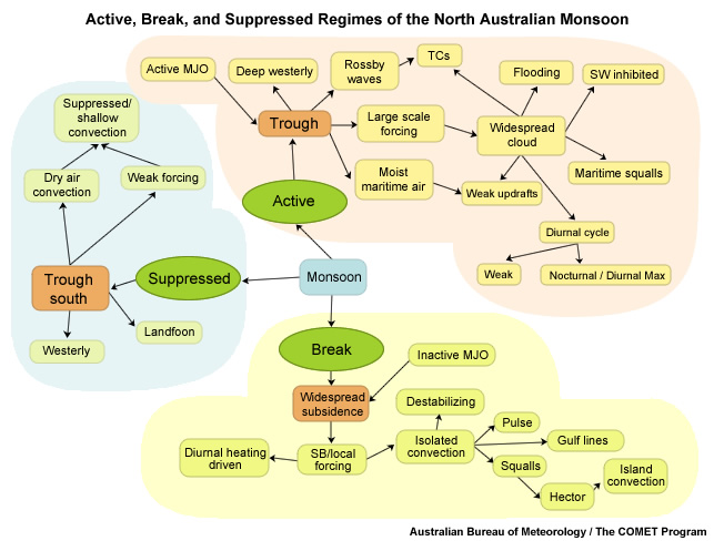
Figure 9F1.28 shows a summary of the major features of the NAM. Like the Indian monsoon, the NAM undergoes alternating active and break monsoon periods with the migrating monsoon trough. The location of the trough exhibits an inherent transient nature but is also modulated by the MJO and equatorially trapped waves such as Rossby waves.
During the active monsoon, there is large scale forcing due to the monsoon trough, advecting a deep westerly, moist maritime air mass. Widespread cloud and precipitation occurs with relatively weak convective updrafts. The diurnal cycle is weak, with an overnight and morning maximum in convective activity due to its maritime nature but also an afternoon maximum over land due to boundary layer heating. Weather hazards, apart from tropical cyclones, include monsoonal squalls and flooding due to widespread, persistent rainfall from MCSs.
During break monsoon periods, widespread subsidence means that convection is forced locally on sea-breeze boundaries and is largely diurnal in nature. Short wave heating of the surface and long wave cooling of the mid troposphere contrast to the cold pool driven cooling of the surface and latent heating of the mid troposphere during the active monsoon. The result is isolated but more intense deep convection during the break period in the form of pulse convection, and various propagating lines of convection such as continental squall lines and Hector.
A third regime of the monsoon occurs when the monsoon trough is found in central Australia. Under these conditions, dry air wraps around a deep low, sometimes in the form of a “landfoon”, resulting in dry westerly winds over northern Australia and convectively suppressed conditions.
Focus 2: The Tropical Forecasters' Perspective
In order to understand how a tropical cyclone forecast is created, we interviewed two forecasters from NOAA's NHC (RSMC with responsibilities for the North Atlantic and Eastern Pacific) and one forecaster from Météo-France La Réunion (RSMC with responsibility for the South Indian Ocean). They also tell us about the path they took to tropical cyclone forecasting and changes in the forecast process during their careers.
Focus 2: The Tropical Forecasters' Perspective »
9F2.1 National Hurricane Center Forecasters (Audio Interviews)
Audio interviews were conducted with the NHC forecasters, Dr. James Franklin and Dr. Lixion Avila, on 9 June 2009. Here are edited versions of those interviews.
Dr. James Franklin
Question 1
How and when did you decide to become a tropical cyclone forecaster? What was your path? Did you do anything special in elementary or high school to further your goals?
Answer:
The path really began as a 6 year-old experiencing Hurricane Cleo when it went over my house, … but that's really what triggered my interest.
I didn't start out in forecasting at all. I was a researcher for 17 years, flying into storms with the hurricane research division of NOAA; did some operationally related research towards the end of that period when the GPS dropwindsonde got developed and spent some time looking at how hurricane winds behaved, the structure of those winds with height in the eye wall. That work caught the attention of some of the folks at the National Hurricane Center and they actually approached me about whether I had some interest in doing it. I hadn't really thought about it at all until they talked to me about it.
A lot of things in life I think are fortuitous. Being exposed to some hurricanes growing up; while I was in school at MIT, Bob Burpee who was at the Hurricane Research Division, was on sabbatical. I took his course on tropical meteorology, I guess I did well enough to have him approach me about a position.
All through high school, I had two main interests: one was meteorology the other was astronomy. Meteorology seemed to be the more interesting field, at least had more of an influence on people's lives and was a little bit more exciting. So that was the field I ended up taking. But I knew that going into college, that that's the kind of thing that I wanted to do, weather in general, I didn't know it was going to be hurricanes at the time.
I did spend a fair amount of my undergraduate time at MIT taking meteorology with folks like Fred Sanders, Pauline Austin, and spent some time with Fred, Kerry Emanuel going back and forth across the New England coastal front in Fred's Rabbit. My master's thesis was going to be on the New England coastal front. My good friend, Frank Marks, who was at MIT at the time, agreed to look over the collection of the data, while we went out and took the observations. Came back and found out the Frank had erased all the data instead of saving it and I was left with no thesis. Bob Burpee took me at the Hurricane Research Division anyway. A couple of years later, we came up with another thesis topic.
Question 2
What process do you use to forecast TC? What tools? Does your answer differ between track, intensity, size and rainfall forecasts?
Answer:
Track
Many years ago people could outfox the guidance at least in terms of track forecasting, but the numerical models have gotten so much better over the last 15, 20 years, in fact, our track forecasts are now about twice as good as they were 15 years ago. It's really very difficult for a forecaster to out integrate numerical models.
A very powerful technique in all of meteorology not just hurricanes is the idea of consensus. Get 3 or 4 or some group of skillful numerical models and you combine them. That's our goal; every time we sit down to make a forecast, that there is something that we can add to try and improve on that consensus. Is there a model that isn't initialized well? Do we recognize a situation when a certain model tends to perform well or tend to perform less well in? Very often your expectations for intensity play into the track forecast, but it all centers around the notion of a consensus and then trying to make moves in one direction or another from that.
One aspect of the forecast process has to do with presenting a consistent picture to our users. We have a very strong continuity constraint from one forecast to the next. We tend to make small increments on the forecast that came before us, improve what you inherited. I haven't talked about intensity so let me go on to that a little bit.
Intensity
Intensity forecasting is a little bit different then the track forecasting in the sense that guidance is not nearly so advanced. The forecast on the other hand does a better job than our intensity guidance. We have 4 intensity guidance models, 2 are dynamical, and 2 are statistical. The human forecaster can see a lot more of what's going on with the storm in terms of its convective structure and how the wind field is organized in terms of concentric eyewalls. None of the kinds of core factors is really well incorporated into our existing intensity guidance. By seeing what's going on in the core, that's where it is the forecaster really adds value to the guidance and is able to contribute a lot more to the process.
Size
We also forecast the size of tropical cyclones to issue these wind radii forecasts, the maximum extent of hurricane force winds in each of 4 quadrants around the center. So we are actually ahead of ourselves there in terms of what we provide relative to what we can do skillfully. So our error in even estimating that parameter is on the order of 50%. That a really tough one. About all that we have to help us with those are climatology and persistence models, the CLIPER model for example for wind radii. We have presumption that as a storm strengthens generally is it going to larger. After a storm is complete, we do what's called a best track, a post analysis of all the available data to create a permanent record, our best record of what happened with that particular storm: location, pressure, maximum sustained wind speed and the status, whether it's a tropical, subtropical, extra tropical. Until very recently we did not do a best track on the wind radius. Until you get to 2004, 2005, those are all operational estimates. They were not reviewed after the fact, those data certainly are not the same quality as the final best track intensity estimates. We've also got very few, sometimes no, real measurements of how large these radii really ought to be. From looking at the cloud shields, surface observations (these are very few), we have some additional tools to help us there. The AMSU, microwave instrument also gives us some size estimates.
Rainfall
Responsibility for rainfall forecasts lies with the Hydrometeorological Prediction Center. They are looking at model guidance, analogs, and previous storms. In our advisories now, we get the guidance for rainfall from HPC.
Question 3
Have ensemble model predictions changed your process?
Answer:
Ensembles are a big part of the tropical cyclone forecast process. Two primary methods would be to take a single model and run it repeatedly using slightly different initial conditions. That's one way. That has not been very successful in operational tropical cyclone forecasts. You can also form a consensus from different models.
When the members that make up an ensemble are independent you get a much better ensemble mean. We're also finding for intensity forecasting, if you form a consensus of the four main intensity models, it is much better on average than any of those four models individually. I think part of the reason for that is those models are very independent. They're not even the same type, you have two statistical models and you have two dynamical models and they're quite independent and it's that independence that really helps you. When members of an ensemble are independent, the errors tend to cancel, particularly when the synoptic situation is relatively simple, so we see this a lot in the eastern Pacific when the synoptic flows are simple. A lot of the errors in the models are random so if you can combine 3 or 4 of them you get a much better forecast then any individual one.
In the Atlantic the signal is not so strong. In the Atlantic we have stronger synoptic scale forcing, more complicated environments, midlatitude troughs coming down and a lot of other features in the environment and in that situation the different models are handling these features in different ways. The consensus concept in the Atlantic is a little bit less effective than it is in the east Pacific because there is more of a systematic component to how the models behave.
Question 4
What's your day like when there is a TC to forecast? How is it different if there are a number of TC? Is it any different if the TC are in different basins or in the same basin?
Answer:
Forecasting shifts are divided in to three: day, evening and midnight shifts. The day shift is responsible for 2 forecasts at 11:00 AM and 5:00 PM. The evening shift is responsible for the 11 PM advisory. The midnight shift is responsible for the 5:00 AM advisory. The day shift is longer, more tiring, much more hectic with more people floating around and more of a media presence.
The forecast cycle basically runs for 3 hours. The 11:00 AM advisory, for example, starts at 8:00 AM with an aircraft reconnaissance fix. You spend about 15 minutes analyzing the data from the reconnaissance aircraft, initial location, initial intensity, initial motion, initial size, all the parameters that are going to go into initializing the numerical model guidance. You update the best track and then submit guidance. We get it back and from about 8:30 AM and in this case up until 10:00 AM is spent making the forecast, looking at the models, the guidance, water vapor imagery, sea surface temperature all the different parameters that are important to track and intensity. By 10:00 AM you have your forecast prepared and we do a conference call with other weather service forecast offices as well as other agencies in the federal government. HPC will be on there, to talk about rainfall; the Storm Prediction Center will be on there, to talk about tornado threats; the Navy is there; Homeland Security is there; a whole host of agencies are there where we discuss the forecast, coordinate any issues that need to be coordinated, like where watches and warnings might be. That call can last from 3 or 4 minutes to a half an hour.
After the conference call is done we then prepare the forecast. We write our discussions and a summary of our rational behind the forecast. We talk about things like forecast uncertainty, why we've analyzed it to be the intensity that we have, why we've chosen the forecast that we have. That's a very important product for us used by emergency managers, the general public helps to provide some context for the forecast. In that last 45 minutes we're writing the discussion, we're preparing the public advisory.
If there are multiple storms you may have to do that for two and on occasion I've had to write even three advisories at once in that three hour period. We do have 2 forecasters on shift, but sometimes we may be working as many as 5 storms simultaneously between the Atlantic and east Pacific. There are times where you really have to compress it. It really depends on what kind of storms you have to deal with. If we have a significant landfall going on or imminent, within a couple of days of landfall, one of the forecasters will focus on that storm exclusively and leave 2 or even 3 to the other person if they are a less difficult forecast situation. We will try, when we have more than 3 systems, to bring in somebody to help us out. They are called hurricane support meteorologists; they have some experience in putting together advisory packages. They come in and help us with the least complicated of the systems that we're working on so that folks from the marine tropical forecasting unit, they're the folks that do the marine forecasting, or they might be from the technical support branch here at the hurricane center. They do have meteorology degrees, so some of them do have experience writing advisory packages. They're all Hurricane Center employees.

Dr. Lixion Avila (English)
Question 1
How and when did you decide to become a tropical cyclone forecaster? What was your path? Did you do anything special in elementary or high school to further your goals?
Answer:
I wanted to be a hurricane forecaster since I was a kid in Cuba and I was always asking questions to the farmers and to the fishermen. But, actually, I didn't start doing that until I was able to finish what you call pre-university degree in Cuba. I entered the Met Service in Cuba but I always wanted to be a hurricane forecaster. After that I went to the United States and I got my Masters and Ph.D. and I was lucky enough to enter the National Hurricane Center and I've been a forecaster for almost 25 years.
I got my degree in Cuba and I worked as a forecaster. But you take care of all the weather systems including hurricanes and I did that for about 5 years.
What I didn't know when I was in elementary school is that you needed a lot of math and physics to study meteorology but actually I love math and physics so it turned out to be good. That's one of the things that really got me by surprise. When you're a kid you don't know that you need those tools, you thought it was more like a fun thing to do than really study hard.
When I was a little kid, one of the things that I enjoyed was to wait for the afternoon thunderstorms, especially in the hurricane season. I grew up near the beach so there was some hills in between the ocean and the beach. Sometimes, I see the thunderstorms coming from south and sometimes I see the storms coming from the ocean. And it was really wonderful for me to enjoy the development of the clouds. And it was really interesting to see that. I am glad that my parents put up with that and they always pleased me with that craziness. But it turned out to be the best for me in the world.
Question 2
What process do you use to forecast TC? What tools? Does your answer differ between track, intensity, size and rainfall forecasts?
Answer:
I've been doing this since 1971. I have seen how the tools have changed. Tremendously! In the '70s we were plotting the surface data by hand. We were getting, maybe, one map a day of a forecast of 24 hours at 500 mb. The facsimile; we even got 1 satellite picture or two satellite pictures a day. And that was probably the case in most of the Caribbean countries and probably not very different in the United States.
We began to get more and more satellite pictures…What really changed the way of forecasting is the development of numerical models and computer science. And, nowadays, we can use all these sophisticated computer models and the physics and dynamics that goes into models to predict hurricanes.
First thing we do in the morning, is to look at the entire globe and all the satellite pictures and look at the different systems. Then we emphasize the system that we think is going to do something or not. We look at the analysis of what's going on through the computer models, of course, using the, also, the conventional data. Before I wasn't able to integrate in my head 5 days in advance, now the computer models are able to give me a better estimate, at least, what could happen, or the possibilities that could happen in terms of the distribution of high pressures and low pressures.
Nowadays we make a 5-day forecast and the weather pattern that is going to affect that cyclone today, if it's in the Caribbean, that weather system is, perhaps, in the western Pacific now, then move to the east. So we need to look at the whole pattern. Either track or intensity, you have to look at the whole thing because the intensity change is related to, perhaps, an upper trough coming. It is more difficult, of course, the forecast of the intensity.
Size
At this moment when we make a prediction, if we don't have data, we don't even know the size of the system. So what we do is try to extrapolate. But we don't have any tools to predict changes in size other than climatology. Perhaps some of the numerical models would give us the size of the storm when they are moving and becoming extratropical in higher latitude. The models are doing a little better, but in terms of the deep tropics the change and size, it's very difficult to predict. What we do is just basically use extrapolation and when we get new data that tell us that the size is larger, we adjust with the new data.
Rainfall
In terms of rainfall, it's even more difficult. Rainfall is probably the cause of most of the deaths, for example, in the region of the Caribbean. But it's the same in most of the tropics when you even have a small, weak tropical depression that could produce 20 inches of rain and produce a tremendous amount of damage. And, unfortunately, many people are killed by the rainfall, especially by flash floods and all this orographic rain that you have when you have a weak tropical depression. Those are very difficult, difficult processes, both the size and the rainfall.
You know, the intensity of a tropical cyclone has nothing to do with the rainfall. It's basically the speed and the amount of convection that the system has. You can have a hurricane that can produce less rain then a weak tropical depression.
There are some old rules I learned from the old-timers and they use the number 100 divided by the speed of the tropical cyclone and you get the amount of inches of rain. And it's so interesting to see that some models, like the GFDL and others, when you compare with that rule the numbers on average turn out to be very close. The bottom line is that it's the speed of the system what matters.
Question 3
Have ensemble model predictions changed your process?
Answer:
Here at the National Hurricane Center, what we have been using is another type of ensemble. What we call the "consensus", which is not just the ensemble of one model but the consensus of different models. And, actually, that turns out to be one of the best ways of making a forecast. It appears that, when you make the consensus of different models, you cancel all the biases of the models and you end up having a better forecast by using all these consensus models.
Yes, it changed the process and makes my life, I would say, a little bit easier. But, still, you have to understand why each particular model is doing what it's doing. You cannot use models as a black box, you have to understand what goes into each model.
In many cases here, when we do the verification, the forecaster turns out to be better than all the different independent models. Because we are using all the information and we process it and we get, as I mentioned, we understand the strength and weakness of each model and we try to improve on that.
Question 4
What's your day like when there is a TC to forecast? How is it different if there are a number of TC? Is it any different if the TC are in different basins or in the same basin?
Answer:
Things have changed too, throughout the years. I do remember when we were 5 hurricane specialists and I have to do almost all of them. And now, luckily, we have more specialists and we get help from other colleagues here at the National Hurricane Center. We are prepared to have simultaneous tropical cyclones. Of course, the pressure is tremendous, especially if you have a hurricane that is threatening land areas. If it's a strong hurricane, we have to take care of the media. But, our emphasis is to be able to get all the information and try to make the best forecast possible.
Do I get nervous? No. Do I get excited? Yes! I do get very excited. I have to be in control, but always, what I like to do is emphasize on the science. I don't want to be biased by any of my feelings and I want to do the best job possible. But, it's a very interesting day. It's a very interesting day when you have a tropical cyclone. I presume that it is the same with a doctor when they have somebody that they want to cure or they want to improve their health. I want to make the best forecast.
I've been offered to work for insurance companies. I have been offered to work for TV. But, there is something about being here at the National Hurricane Center; that I have the "power" to name a system. You might think it's not important, but for me, it kind of means that I'm on top of the science and I'm doing this. For me, it's one of the fun things that I get from the job.
| Dr. James Franklin |
Question 1How and when did you decide to become a tropical cyclone forecaster? What was your path? Did you do anything special in elementary or high school to further your goals? Click Question 2What process do you use to forecast TC? What tools? Does your answer differ between track, intensity, size and rainfall forecasts? Click Question 3Have ensemble model predictions changed your process? Click Question 4What's your day like when there is a TC to forecast? How is it different if there are a number of TC? Is it any different if the TC are in different basins or in the same basin? Click |
Dr. Lixion Avila (English) |
Question 1How and when did you decide to become a tropical cyclone forecaster? What was your path? Did you do anything special in elementary or high school to further your goals? Click Question 2What process do you use to forecast TC? What tools? Does your answer differ between track, intensity, size and rainfall forecasts? Click Question 3Have ensemble model predictions changed your process? Click Question 4What's your day like when there is a TC to forecast? How is it different if there are a number of TC? Is it any different if the TC are in different basins or in the same basin? Click |
Focus 2: The Tropical Forecasters' Perspective »
9F2.2 Tropical Cyclone Centre Météo-France, La Réunion
Interview with Dr. Anne-Claire Fontan, tropical cyclone forecaster
1. How and when did you decide to become a tropical cyclone forecaster? What was your path? Did you do anything special in elementary or high school to further your goals?
I became a tropical cyclone forecaster at the RSMC/Tropical Cyclone Centre Météo-France/La Réunion 12 years ago, once I finished studying at the French school dedicated to meteorology “ENM” (Ecole Nationale de la Météorologie de Météo-France / Météo-France National School of Meteorology), located in Toulouse, France. This school gives a diploma in meteorology, which takes three years to complete (after either two years in a university-level college, or a Master of Science at the university).
Before this school, I was at university where I studied for a Masters degree in oceanography and meteorology at Marseille and Paris. In France, there is no way to specialize in meteorology until you have completed a bachelor or Masters degree or the “ENM”, but you need to choose a scientific path from high school.
Once you have graduated, and got the job at the RSMC/TCC La Réunion, you have to follow an extra two weeks formation in tropical meteorology. Afterwards you become a “trainee” in operations during several months at the RSMC. During this period you are given an additional formation and practice through tutoring with experienced TC forecasters. A TC forecaster is considered to be accomplished after one or two complete cyclonic seasons.
2. What process do you use to forecast TC? What tools? Does your answer differ between track, intensity, size and rainfall forecasts?
To forecast at the RSMC/La Réunion, we use a powerful workstation called SYNERGIE. This workstation displays and superimposes all the data a forecaster needs to work: observations, models, satellite imageries, radar, etc. There is a specific module dedicated to tropical cyclones called SYNERGIE CYCLONE which allows us to focus on tropical cyclone analysis and track and intensity forecasts. In addition to models, observations, images, and TC tracks plots, we have recently implemented the possibility to display directly the websites data we use daily in operation. These websites are mainly – and so not exhaustively - the tropical cyclones pages from the NRL, the CIMSS, the NOAA (QuikSCAT), the AOML (heat potential), the Australian BoM (MJO), ….
Our area of responsibility (Equator to 40°S and African coastline to 90°E) is mainly a maritime basin, except the western part between African coasts and 60°E. We rely indeed a lot on satellite data. Size and rainfall associated to the systems are “observed”, not yet specifically forecast. Every 6 hours, as we issue our warnings, we describe the size of the TC, based on the 30 knots and 50 knots winds, by using all the available observations; these are mainly received through scatterometer data - due to the maritime characteristic of our basin. We also describe the weather and the rainfall associated with the system. When a TC is forecast to approach or hit a landmass the “comments part” of the warnings specifies as well the inhabited areas the rainfall can concern in the next 24 to 36 hours. In this case, we use forecast fields as the precipitation rate, humidity, vertical velocity, …, of the best model.
Track forecast
We get the fields from the numerical models developed by different countries/centres to be able to track forecast; two models from Météo-France, a global one and a limited area one (over Southern Indian Ocean), one from the UKMO (United Kingdom Met Office), and the Ensemble Prediction System (EPS) average and the deterministic models from the ECMWF (European Centre). Since season 2004-2005 we get as well the “geopoints” (i.e. position and MSLP (Mean Seal Level Pressure) of the TC each 6 or 12 hours) of some of the American numerical models via the JTWC; GFDN, NOGAPS, AVNO, and consensus of different models computed at the JTWC. These models tracks are displayed on the workstation.
Thanks to the analysis of the fields from the models, the forecaster decides which scenario is the best. Afterwards, as statistics tend to show consensus of models lead to the better results, we average chosen models to make the track forecast. If philosophy of some of the models totally differs from the chosen one, we do not involve them in the average.
Intensity forecast
To forecast intensity, we need to know the current and follow-on environment of the system. Several tools are used. We study the products of the CIMSS to get the current environment and to get it for the few hours to come; upper level divergence and winds, low level convergence and winds, wind shear, shear tendency, and so on. We get the heat content thanks to the SSTs satellite data and the AOML website heat potential (depth of the 26°C isotherm). Humidity is assessed thanks to WV and MW imageries. Then we use the fields of the model estimated to be the best for the situation: θ’w at 700 hPa, divergence, convergence. And we have a look on the tendency of the different models, if ever they deepen or weaken the system.
3. Have ensemble model predictions changed your process?
For the past few years we received data from the Ensemble Prediction System (EPS) and it has changed the way we work and our results. We use it to further several goals. First of all, the EPS is used to assess the probability of cyclogenesis over the basin for the 10 coming days. Then the average of the 51 runs of the EPS is used as a ”deterministic model” and can be involved into a consensus of models to make the TC track forecast. Strike probabilities provided on each system by the ECMWF is used to manage the risk at La Réunion Island. The last goal, still under investigation, would be to use the EPS to provide cones of uncertainty for the RSMC forecast track.
4. What’s your day like when there is a TC to forecast? How is it different if there are a number of TC? Is it any different if the TC are in different basins or in the same basin?
We work in 12 hour shifts either day or night. These shifts range between 7.00 AM to 7.00 PM and 7.00 PM to 7.00 AM. We issue four series of warnings a day at 00, 06, 12, 18Z. So for example, for a day shift we have the 06 and 12Z warnings to issue.
At first we have the changeover and a detailed study of the current situation. At 08.30 AM we have the briefing for the people working at the centre. Straight afterwards starts the entry of the data in the software we use to prepare the 6 or 7 warnings which will be issued in both English and French at 10.30 AM (0630Z). Then we brief the local weather forecast service and if necessary (i.e. if the TC directly or indirectly concerns the weather on Réunion Island), we provide it with guidance and directives. We have a break between 11.00 AM and 12.00 PM.
Afterwards, we have a database dedicated to cyclogenesis to fill in, and the writing of the tropical weather outlook in both English and French, which will be issued at 03.00 PM. Meanwhile we write the “connection bulletin” which allows to keep the information within the team, and to give instruction for the three following days to the local forecast team.
The following warnings are prepared and issued at 04.30 PM. At the end of the shift, we have to update the archives of the day with messages, pertinent satellite images, and so on.
When there is a risk to manage on Réunion Island, we issue some extra warnings at 1.00 PM and 7.00 PM for the local authorities and for the public, and we answer to the media.
If ever there are two TC to deal with, it is double the workload! If there are two systems to monitor, with a risk to manage on the Island, a second cyclone forecaster comes to help. We get somebody in extra as well if ever there are more than two systems over the basin.
We have a single basin to monitor. But this basin has a “virtual border” with two others ones; the south-east Indian Ocean (the Australian area of responsibility starts at 90E) and the Indonesian area of responsibility (east of 90E, north of 10S). If ever a TC comes from one of their areas of responsibility to ours or vice versa, the different centres (Perth, Jakarta and Réunion Island) send e-mails or phone to manage the handover.
Focus 2: The Tropical Forecasters' Perspective »
9F2.3 Météorologique Régional Spécialisé / Centre des Cyclones Tropicaux de La Réunion, Météo-France
Entretien avec Anne-Claire Fontan, ingénieur prévisionniste cyclone
1. Comment et quand avez-vous décidé de devenir un prévisionniste cyclone? Quel a été votre cursus? Avez-vous suivi un parcours spécifique que cela soit en primaire, collège ou lycée pour atteindre votre but?
Je suis devenue ingénieur prévisionniste cyclone au CMRS/ Centre des Cyclones Tropicaux de La Réunion il y a 12 ans, une fois mes études terminées à l’ENM (Ecole Nationale de la Météorologie), l’école d’ingénieurs dédiée à la météorologie, dépendant de Météo-France, et située à Toulouse, en France. Cette école délivre un diplôme en météorologie qui nécessite trois ans d’étude ( qui viennent après deux ans de classes préparatoires aux grandes écoles ou une maîtrise de sciences de l’université). Avant l’ENM, j’ai fait mes études dans les Universités de Marseille et Paris pour obtenir un Master d’océanographie et de météorologie. En France, il n’est pas possible de se spécialiser en météorologie avant l’université et le niveau licence ou maîtrise -ou avant d’aller à l’ENM, mais il est toutefois nécessaire de choisir une filière scientifique dès le lycée.
Une fois diplômé et une fois obtenu le poste au Centre des Cyclones Tropicaux de La Réunion, il faut suivre deux formations supplémentaires; une première formation théorique de deux semaines en météorologie tropicale à l’ENM, puis une deuxième formation, opérationnelle, pendant plusieurs mois, au Centre des Cyclones. Cette période consiste à travailler avec et sous la supervision d’ingénieurs prévisionnistes cyclone expérimentés. Un prévisionniste cyclone est dit confirmé après avoir travaillé pendant une ou deux saisons cycloniques complètes.
2. Quelle(s) méthode(s) utilisez-vous pour prévoir les cyclones tropicaux (CT)? Avec quels outils travaillez-vous? Si l'on distingue les prévisions à effectuer: trajectoire, intensité, taille ou précipitations, vos réponses sont-elles différentes?
Pour élaborer les prévisions au Centre des Cyclones de La Réunion, nous utilisons une puissante station de travail appelée SYNERGIE, sur laquelle nous pouvons visualiser et superposer toutes les données dont un prévisionniste a besoin pour travailler: observations, modèles, imageries satellite, radar, etc. Cette station de travail possède un module spécifiquement dédié aux cyclones tropicaux (SYNERGIE CYCLONE), avec lequel nous travaillons pour procéder à l’analyse du système tropical et établir les prévisions de trajectoire et d’intensité. En plus des modèles, observations, images et tracé des trajectoires issues des modèles numériques …, nous avons récemment installé la visualisation directe des données des sites Internet utilisés quotidiennement en opération. Ces sites sont principalement – et donc de manière non exhaustive- les pages dédiées aux cyclones tropicaux du NRL, du CIMSS, de la NOAA (QuikSCAT), de l’AOML (pour le contenu énergétique), du BoM australien (MJO), ….
Notre zone de responsabilité (de l’équateur à 40S et des côtes africaines à 90E) est essentiellement un domaine maritime, exceptée la partie ouest du bassin, entre les côtes africaines et le 60E. Nous dépendons donc fortement des données satellitaires.
La taille et les précipitations associées aux systèmes tropicaux sont « observées », mais ne sont pas encore spécifiquement prévues. Toutes les six heures, lors de la diffusion de nos bulletins, nous décrivons la taille des systèmes via l’extension des vents à 30 nœuds et 50 nœuds, essentiellement grâce aux données des diffusiomètres (du fait du caractère maritime du bassin). Nous décrivons également le temps et donc les précipitations associées au système. Lorsqu’un système tropical est prévu approcher ou frapper une terre, la partie « commentaires » de nos bulletins spécifie de plus les zones habitées que les précipitations peuvent concerner dans les 24 à 36 prochaines heures. Pour ce faire, nous utilisons les champs prévus comme le taux de précipitation, l’humidité, la vitesse verticale, …, du meilleur modèle.
Prévision de trajectoire:
Pour élaborer nos prévisions de trajectoire, nous disposons des champs des modèles numériques développés par différents pays ou centres; deux modèles de Météo-France, un global et un à aire limitée sur l’Océan Indien Sud, le modèle anglais du Met Office, le modèle déterministe et la moyenne de la prévision d’ensemble du Centre Européen de Prévision (CEP). Depuis la saison 2004-2005, via le JTWC, nous avons également accès aux « géopoints » (i.e. position et pression minimale au centre du système tropical, toutes les 6 ou 12 heures) de quelques-uns des modèles américains comme le GFDN, le NOGAPS, le AVNO, et consensus de modèles calculés au JTWC. Les trajectoires proposées par tous ces modèles sont visualisées sur la station de travail.
Grâce à l’analyse des champs des modèles, le prévisionniste décide quel scénario est le meilleur. Par la suite, comme les statistiques tendent à montrer que les consensus de modèles mènent aux meilleurs résultats, nous moyennons les modèles choisis pour élaborer la prévision de trajectoire. Si la philosophie de certains modèles ne correspond pas à celle retenue, nous ne les incluons pas dans la moyenne.
Prévision d’intensité:
La prévision d’intensité nécessite la connaissance de l’environnement du système et son évolution. Nous utilisons pour ce faire plusieurs outils. Nous étudions les produits du site du CIMSS pour connaître l’environnement; la divergence et les vents d’altitude, la convergence et les vents de basses couches, le cisaillement vertical de vent et sa tendance, etc. Nous regardons le potentiel énergétique océanique via les températures de surface de la mer données par l’imagerie satellite et le contenu énergétique du site de l’AOML (profondeur de l’isotherme 26°C). L’humidité est évaluée grâce aux imageries vapeur d’eau et micro-onde, et nous utilisons également les champs du modèle estimé être le meilleur; θ’w à 700 hPa, divergence, convergence. Pour finir, nous regardons la tendance donnée par les modèles, s’ils creusent ou affaiblissent le système tropical.
3. La Prévision d'Ensemble a-t-elle changé votre méthode de travail?
Nous somme destinataires des produits de la Prévision d’Ensemble (PE) depuis plusieurs années et cela a changé notre façon de travailler et nos résultats. Nous l’utilisons à différentes fins. Tout d‘abord, la PE est utilisée pour évaluer la probabilité de cyclogenèse à 10 jours sur le bassin. Ensuite, la moyenne des 51 runs de la PE est utilisée comme un modèle déterministe et peut être incluse dans un consensus de modèles pour élaborer la prévision de trajectoire. Le panache de probabilité (« strike probabilities ») fourni par le CEP sert à la gestion du risque sur l’Ile de La Réunion. Enfin, la dernière application, toujours à l’étude, serait d’utiliser la PE pour calculer des cônes d’incertitude appliqués à la prévision de trajectoire du CMRS.
4. Comment se déroule une journée de travail lorsqu’un système tropical évolue sur le bassin? En quoi est-ce différent s’il y a plusieurs systèmes tropicaux à la fois? Suivant si les systèmes tropicaux évoluent sur le même bassin ou bien sur des bassins différents, cela fait-il une différence dans votre journée de travail?
Nous travaillons selon des tours de service de 12 heures, qui peuvent être de jour ou de nuit. Les horaires de ces tours de service sont de 07h00 à 19h00 et de 19h00 à 07h00. Nous émettons quatre séries de bulletins par jour, en français et en anglais, à 00, 06, 12 et 18Z. Nous avons donc lors d’une journée de travail, les bulletins de 06 et 12Z à élaborer et diffuser.
La journée commence avec la relève et l’étude approfondie de la situation, exposée lors d’un briefing pour le personnel du centre à 08h30. Nous enchaînons avec la saisie de données dans le logiciel avec lequel nous préparons nos 6 à 7 bulletins, qui sont diffusés en bilingue pour 10h30. Vient ensuite le briefing interne avec le service de prévision du temps local et si nécessaire (i.e. si un CT concerne directement ou indirectement le temps sur La Réunion), nous lui fournissons des directives.
Nous avons une pause entre 11.00 AM et 12.00 PM.
Après cela, nous devons remplir une base de données concernant la cyclogenèse, et débuter la rédaction du bulletin en anglais et français sur l’activité cyclonique et les conditions météorologiques du bassin (« tropical outlook »). Ce bulletin est diffusé à 03h00. Entre-temps, nous élaborons le bulletin dit de « liaison » permettant de tenir l’équipe informée des actions de la journée et de donner des instructions à l’équipe de prévision locale pour les 3 jours à venir.
Les bulletins du réseau suivant sont ensuite préparés et diffusés pour 04h30. A la fin du service, nous procédons à l’archivage des messages, des images satellitaires pertinentes, etc, de la journée.
Si jamais nous avons deux CT à gérer, c’est double travail! S’il y a deux systèmes à suivre, avec une gestion de risque sur La Réunion, un deuxième prévisionniste cyclone vient donner de l’aide. Quelqu’un vient également en renfort lorsqu’il y a trois systèmes à gérer sur le bassin.
Nous avons un seul bassin à surveiller, mais il a une frontière « virtuelle » avec deux autres zones; le sud-est de l’océan Indien (la zone de responsabilité australienne débute à 90E) et la zone de responsabilité indonésienne (est de 90 E et nord de 10S). Si jamais un CT nous arrive d’une de ces deux zones (ou vice et versa), les centres concernés (Perth, Jakarta, La Réunion) s’envoient des mels ou s’appellent pour assurer la passation de responsabilité de suivi du système.
Summary
Tropical weather observation, analysis, and forecasting are challenging but continue to improve thanks to new instruments (mostly satellite and some in situ), derived variables, and tools for synthesizing observations and numerical model output. Forecasters add value to the automated systems using their knowledge of model biases, rapidly updated satellite information, and past cases. Satellite data analysis is one of the most critical skills for tropical weather forecasters. Since radars are sparse in the tropics, high resolution geostationary images aid in nowcasting mesoscale and convective-scale weather systems. High resolution, non-hydrostatic models are producing realistic convective weather systems at many scales, however, data assimilation methods are challenged by increasing amounts and types of satellite data. Ensemble techniques are providing information on model forecasts uncertainty. Multi-model ensemble (consensus) models have led to better tropical cyclone track forecasts. While tropical cyclone intensity forecast skill is lagging, ensembles of statistical and high-resolution dynamical models provide the best numerical guidance currently. Intraseasonal forecasting is becoming mature enough to be used as guidance for the probability of tropical cyclogenesis. New and traditional forecast verification and validation techniques are helping tropical forecaster evaluate numerical forecasts. As knowledge of tropical meteorology and confidence in NWP increases, we expect to see more improvements in tropical weather forecasting.
Appendix A: Station Plot and Weather Symbols
Surface station data are plotted at its location on a weather map in a format shown in Fig. 9A.1. To the upper right is mean sea-level pressure (MSLP); the leading digit(s) is dropped (9 or 10 in the case of MSLP). Therefore, a MSLP value of 998.6 hPa is plotted as “986” while 1011.5 is plotted as "115". The circle shows the sky cover in eighths or oktas (Fig. 9A.2). The wind barb represents speed and the direction from which the wind is blowing. For standard upper-air horizontal analyses (1000, 850, 700, 500, 300, 200 hPa), the station plots show temperature, dewpoint, wind velocity, and geopotential height. A sample 850 hPa data plot is shown in Fig. 9A.1b, where geopotential height of 1564m is plotted as “564”. Other commonly used weather symbols are shown in Fig. 9A.2.
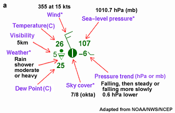
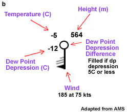
Questions for Review
- Describe at least two challenges that are unique to tropical weather forecasting.
- List three types of point measurements.
- List three sources of observation error.
- What are the advantages and weaknesses of satellite observations when compared to station observations of the tropics?
- Describe two advantages and two limitations of weather radar observations for tropical weather analysis and forecasting.
- Why is streamline/isotach analysis more useful for tropical weather forecasting than isobaric analysis?
- List at least two instruments (in situ or remote-sensing) developed for research that have been applied to tropical weather forecasting since the 1990s.
- How does monitoring intraseasonal circulations, such as equatorial waves and the MJO, help tropical forecasters?
- List uses and limitations of trajectory analysis for tropical weather forecasting.
- List three variables forecasted for tropical marine weather.
- Describe how satellite and radar images are used to analyze the evolution of tropical mesoscale convection.
- Describe at least four sources of numerical weather prediction model error.
- What is the purpose of data assimilation?
- What are the fundamental principles represented by the “primitive equations” used in dynamical models?
- Why are non-hydrostatic models better for tropical weather prediction than hydrostatic models?
- Explain what constitutes an ensemble numerical forecast.
- Describe the advantages and limitations of three-dimensional (3D-VAR), four-dimensional variational (4D-VAR), and Ensemble Kalman Filter data assimilation techniques.
- Describe three methods for verification of NWP model forecasts including their strengths, weaknesses, and at least one example of their application in tropical weather.
- List three factors that must be considered when forecasting tropical cyclone motion.
- List three factors that must be considered when forecasting tropical cyclone intensity change.
- When are statistical models most useful in tropical cyclone forecasting?
- What are some of the key physical variables included in a typical statistical model used for tropical cyclone forecasting?
- Give a basic description of two dynamical models used for tropical cyclone motion forecasts.
- When are ensemble techniques most useful for tropical cyclone prediction and why?
- Describe two techniques used to validate tropical cyclone motion or intensity forecasts.
- List the major differences between active and break monsoon periods over Northern Australia in terms of dynamics and thermodynamics.
- Describe the differences in the diurnal cycle of convection between active and break monsoon periods. What impact does this have on aviation forecasting at Darwin, Australia?
- List as many of the severe storm types you can and at least one feature in the radiosonde that would alert you to potential severity.
- Briefly describe why suppressed monsoon periods occur over northern Australia. How are these periods different to the typical active monsoon?
- What role does orography play in the seasonal cycle of precipitation over the Maritime Continent (SE Asia)?
QUIZ
You may also take a quiz and email your results to your instructor.
Brief Biographies
Dr. Akio Arakawa
Dr. Akio Arakawa is a pioneer in global numerical weather prediction (NWP). He received his B.Sc. in physics and D.Sc. in meteorology from Tokyo University in 1950 and 1961, respectively. While working at the Japan Meteorological Agency during the 1950s, he developed his first global atmospheric circulation model, having been inspired by Norman Phillips’s first general circulation simulation. He came to the University of California Los Angeles (UCLA) as a visiting scientist in 1961 after being recruited by Yale Mintz. In 1963 they completed the first UCLA General Circulation Model, which later became known as the Mintz-Arakawa Model. It was the first global model to include realistic land-sea distributions and surface topography. Arakawa returned to UCLA in 1965 after a two-year period in Japan. He remained at UCLA as a faculty member for the rest of his career while leading the development of increasingly sophisticated general circulation and earth system models.
Using his brilliant mathematical skills and meteorological expertise, he developed numerical methods for representing fluid dynamics including finite difference techniques first published in 1966. He also developed robust schemes for representing the interaction of cumulus convection and large-scale circulations, creating with Wayne Schubert, the “Arakawa-Schubert cumulus parameterization scheme” in 1974. These contributions have led to major advances in tropical weather prediction and earth system modeling in general. He received the Carl-Gustaf Rossby Research Medal in 1977, the highest award granted by the AMS. His career was celebrated at UCLA in 1998 with, “General Circulation Modeling Past Present, and Future: A symposium in honor of Akio Arakawa. He was made a Fellow of the AMS and an AMS symposium was held in his honor in 2007. He was a recipient of the UCLA Dickson Award for 2008. Most recently, he was awarded the 2010 Vilhelm Bjerknes Medal by the European Geosciences Union in recognition of his pioneering and fundamental contributions not only to numerical modeling in atmospheric sciences but to geophysical fluid dynamics in general. Although retired, he continues to be involved in ongoing efforts to refine global models including climate models. He is regarded as a “living legend”.
Benito Viñes (1837-1893)
Known as the “Hurricane Priest”, Father Benito Viñes, laid the foundation for the modern observational and hurricane warning network. He was the director of the Magnetic and Meteorological Observatory of the Royal College of Belen in Havana, Cuba from 1870 until his death in 1893. He was born in Poboleda, Spain, received training in physics, and came to Cuba via France. He organized hundreds of observers to monitor weather along the coast of Cuba, thereby establishing the first observational network that delivered hurricane warnings by pony express and later by telegraph. From his meticulous observations of surface weather, cloud motion, sea-swells, and post-landfall assessment, he developed a fairly accurate conceptual model for the three-dimensional structure of hurricanes. By observing cloud motion and sea swells, he also created a technique for finding the center of hurricanes. He became famous for pioneering forecasts of hurricane motion based on the movement of high cloud outflow from the center of tropical storms. In September 1875, he became a legend after he issued his first printed forecast and accurately forecasted the landfall of an intense hurricane in southern Cuba. Subsequent success later that year and in the following years resulted in Viñes gaining funding from private companies to aid with observation stations and free message service from telegraph and railroad companies. He published his now famous Practical Hints in Regard to West Indian Hurricanes in 1877 and it became a standard training resource for mariners and others. His technical report on the Cyclonic Circulation and Translatory Movement of West Indian Hurricanes was delivered posthumously to the U.S. Weather Bureau, having been mailed three days before his death.
Thanks to Patrick Fitzpatrick for sharing biographical information from his book, "Hurricanes; a reference handbook, 2nd Edition", Contemporary World Issues, ABC CLIO, 412pp, 2006.