Table of Contents
- 3.0 Overview
- 3.1 General Principles of Atmospheric Motion
- 3.2 General Circulation of the Atmosphere
- 3.3 Ocean Circulation
- 3.4 The Response to Equatorial Heating
- 3.5 Monsoons
- 3.6 Tropical Circulation and Precipitation Distribution
- 3.7 The Role of the Tropics in the General Circulation
- Focus Areas
- Summary
- Questions for Review
- Brief Biographies
- References
3.0 Overview
The chapter begins with a review of the general principles of atmospheric motion including scale analysis of tropical motions. An overview of the general circulation of the atmosphere and ocean is presented including stratospheric general circulation. Special emphasis is given to the Hadley circulation including its maintenance, seasonal migration, northern and southern hemispheric differences, and the contrast between tropical and midlatitude wind systems. Tropical circulations are examined in a theoretical framework as responses to heating at the equator. Regional monsoons, their conceptual models, seasonal evolution, and variability are explored. Modeling of the general circulation is examined in a focus section.
Print Version
The print version provides a single printable page with all required content.
Multimedia Version
The multimedia version provides structured page navigation.
Focus Areas
Quiz and Survey
Take a quiz and email your results to your instructor.
After completing this chapter, please submit a User Survey.
3.0 Overview »
Learning Objectives
At the end of this chapter, you should understand and be able to:
- Recall the primitive equations of motion and continuity
- Recall hydrostatic equation, hypsometric equation, and thermodynamic energy equation
- Estimate divergence and vorticity from streamlines and isotachs using the natural coordinate system of motion
- Understand basic scaling at low latitudes and balances at low latitudes
- Describe various models of global circulation and mechanisms that create their pattern
- Describe the general circulation in the stratosphere
- Describe the tropical tropopause layer and the role of tropical deep convection in global-scale chemical transport
- Identify the semi-permanent highs and lows in the tropics and subtropics
- Recall the seasonal migration of the tropical circulation systems and hemispheric differences
- Understand and describe the similarities and differences between atmospheric motions in the tropics versus the midlatitudes
- Understand the mechanisms that maintain the Hadley cell and its latitudinal extent
- Describe role of the ITCZ in the general circulation and mechanisms that influence its location
- Describe Ekman transport and upwelling in the ocean
- Recall the global upper ocean circulation mechanisms and the major ocean currents
- Describe the current conceptual model of a monsoon
- Understand the theoretical basis for the Hadley cell and the Walker Circulation as responses to differential heating in the tropics
- Understand and describe how the Asian monsoon evolves
- Compare and contrast the Asian monsoon with other monsoon systems in Australia, Africa, and the Americas
- Describe the major modes of global monsoon interannual variability and some of the factors that influence that variability
- Describe the major factors that lead to intraseasonal variability and break periods in the global monsoons
- Describe the major components of a general circulation model
3.1 General Principles of Atmospheric Motion
3.1 General Principles of Atmospheric Motion »
3.1.1 Useful Simplifications of Force Balances Important to Large-scale Motions
Motion in the atmosphere and the ocean can be considered in terms of Newtonian principles, i.e., force = mass × acceleration. Meteorologists are interested in the acceleration of a parcel of air or rate of change of velocity per unit mass = force. This formulation, in terms of time rate of change, produces the Navier-Stokes equations or equations of motion, which apply to both air and water. The pressure gradient force moves fluid from high to low pressure. When rotation, friction, and gravity are added, the acceleration of motion following a fluid on a rotating planet can be written as:
Acceleration = pressure gradient + Coriolis + effective gravity + frictional forces
 (1)
(1) where  (u,v,w) is the velocity vector (m s-1); p is pressure (Pa); ρ is density (kg m-3); f is the Coriolis parameter, defined as f = 2ΩsinΦ = the vertical component of Ω, the Earth's rotation rate (rad s-1), and with Φ as the latitude; and g is effective gravity (m s-2), a combination of the Earth’s gravitational and the centrifugal forces. The acceleration due to the Coriolis Effect, f k x , is at right angles to the velocity (to the right in the Northern Hemisphere and left in the Southern Hemisphere) and frictional forces, Fr, oppose the motion. D/Dt is the sum of the local rate of change plus advection terms,
 .
.
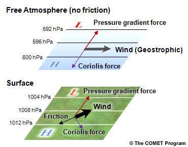
Above the friction layer, balance is between the pressure gradient and the Coriolis force (Fig. 3.1, upper). The actual wind here can be well approximated by the geostrophic wind,  , the wind calculated from this force balance. The wind in geostrophic balance blows parallel to the isobars, which means that these winds are parallel to the other mass fields (density, temperature). This geostrophic approximation holds for large-scale motion away from the equator.a Moving downwards to the surface, frictional forces increase and the surface winds are no longer parallel to the pressure field but angled toward lower pressure (Fig. 3.1, lower).
Flow that is parallel to the isobars around high and low pressure areas results from balance between pressure gradient, Coriolis, and centripetal (negative centrifugal) forces. In these regions near circulation centers the geostrophic wind is not a good enough balance to the observed wind because of the curved flow. The wind calculated from this three force balance is referred to as the gradient wind. While gradient balance exists only near circulation centers, a gradient wind can be defined for the level at which friction is considered negligible; about 2000 ft above the surface.
Vertical motion is expressed as acceleration = pressure gradient + gravity
 (2)
(2) where w is the vertical velocity and g is the acceleration due to gravity (a positive constant, 9.8 m s-2). Since pressure decreases with height, the first term on the right is positive and -g is negative, so the resulting vertical acceleration is determined by their relative magnitudes.
One of the fundamental principles in meteorology is that of conservation; a quantity is conserved except for external sources and sinks. The conservation of energyconservation of energy and angular momentumangular momentum were introduced in Chapter 1Chapter 1. Now we will focus on the conservation of mass, which can be expressed as the continuity equation.
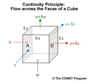
The continuity principle is presented schematically in Fig. 3.2. Consider the rate of transport or flux of air with density, ρ. The rate of flow per unit area moving at velocity of u across area A is defined as ρu. The total flux rate across A into the box = ρu δy δz. The accumulation of mass between faces A and B (situated δx apart) is approximately
 (3)
(3) where δx δy δz is the fixed volume of fluid being observed.
Therefore, dividing through by the parcel volume δx δy δz, the net rate of mass inflow per unit volume can be expressed as  where is the three-dimensional velocity. Since no new mass is being created or destroyed—it is only transported—the mass is conserved. Mass can be flowing out of the volume as well as into it; the net of these is the local rate of change of density in time,
  . Thus, leading to the continuity equation,
 (4a)
(4a)Equation (4a) is known as the flux form of the continuity equation. Expanding the gradient operator and dividing through by ρ, Equation (4a) can be rewritten as
 (4b)b
(4b)bThis second form of the continuity equation (4b) is known as the advective form, since the advection is combined with the time derivative.
The continuity equation is a useful forecasting tool as it relates the rate of density increase of an air parcel to the velocity divergence of the parcel. If the fluid is incompressible, its density is constant in time and the horizontal divergence per unit mass can be calculated by expanding the continuity equation (4b) into its horizontal and vertical components,
 (5)
(5)So it is clear that for an incompressible fluid, horizontal divergence is proportional to change in vertical motion with height. Thus, horizontal convergence (negative divergence) must result in vertical motion out of the volume and horizontal divergence results in vertical motion into the volume.
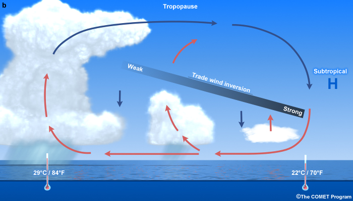
We can use these principles to think about the tropical atmosphere, even though it cannot be assumed to be incompressible: near surface horizontal convergence implies net horizontal flow into the volume and compensating ascent, low pressure, clouds and precipitation. Conversely, sinking motion leads to a surface high pressure, and drying in a region of near surface divergence. In the trade wind regime, sinking motion above the boundary layer suppresses the development of strong thunderstorms, but shallow clouds form at the top of the moist boundary layer. This demonstrates that the response of the atmosphere is dependent on where the divergence/convergence occurs relative to a boundary.
a Coriolis parameter, f, is zero at the equator so the geostrophic wind would be infinite there.
b Recall that is the Eulerian time derivative and is measured at a fixed location (say, your garden).  is the Lagrangian time derivative and measured moving with the parcel. So the difference between these two time derivatives is the advection
  .
.
3.1 General Principles of Atmospheric Motion »
3.1.2 Useful Simplifications for Large-scale Vertical Structure
For synoptic and planetary circulations, horizontal scales are much larger than vertical scales with negligible rates of vertical acceleration or Dw/Dt≈0. Therefore the vertical pressure gradient force is balanced by the weight of the atmosphere. This is known as the hydrostatic approximation or hydrostatic balance and expressed as,
 (6)
(6)Through laboratory experiments, it has been shown that the pressure, density (or specific volume), and temperature of materials can be related by an equation of state, which when applied to gases is known as the ideal gas law. For dry air, the equation of state can be written as
 (7)
(7)where p is pressure (Pa), ρ is density (kg m-3), α is specific volume (ρ-1, so has units m3 kg -1), T is temperature (K), and R is the gas constant for dry air (287 J kg-1 K-1). By substituting for density, ρ, from the ideal gas law, we rewrite the hydrostatic equation as
 (8)
(8)which can be rearranged to show the geopotential, Φ, with respect to pressure, as a function of the temperature, with respect to pressure, as a function of the temperature:
 (9)
(9)By integrating over a layer, we get the hypsometric equation which shows that the thickness of a layer between two pressure surfaces is proportional to the mean temperature of the layer. Pressure decreases more rapidly in a cold column than a warm column as shown by:
 (10)
(10)Because the pressure gradient is related to the geostrophic wind, the mean horizontal temperature gradient in a layer is also related to the geostrophic wind at the top and bottom of the layer. The difference between the geostrophic winds at two levels is proportional to the temperature gradient and expressed as the thermal wind equation, where the thermal wind (VT) is the vertical shear of the geostrophic wind (Vg). So, for the zonal component of the wind, the thermal wind between isobaric layers, p1 and p2 is,
 (11)
(11)where  is the mean temperature in the layer, ug is the zonal geostrophic wind, uT is the zonal thermal wind. This simple dynamical rule, the thermal wind balance, is the most applicable to explaining the average structure of the general circulation. The mean zonal wind is in thermal wind balance throughout the equatorial region.
The atmosphere is also thermodynamically constrained by the conservation of energyconservation of energy; any heat added must be equal to the change in internal energy minus the work done (Chapter 1, Eq. (1)). For an ideal gas, the first law of thermodynamics or thermodynamic energy equation can be expressed as:
 (12)
(12)where Q is the heating rate (J kg-1 s-1) per unit mass, cv is specific heat at constant volume (717 J K-1 kg-1), and cvT is the internal energy. Using cp = cv + R (cp =1004 J K-1 kg-1), we rewrite the thermodynamic energy equation as
 (13)
(13)Then substituting from the ideal gas law (7), we get:
 (13a)
(13a)where Q/ cp is the diabatic heating rate (K s-1 or K day-1).
For adiabatic processes, no heat is exchanged between the system and the environment so Q= 0. Then the thermodynamic energy equation (13a) can be integrated between an initial state (p,T) and a reference state with pressure, p0, and temperature, θ, to obtain
 (14)
(14)where temperature is in Kelvin. Generally p0 is taken to be 1000 hPa and θ is called the potential temperaturepotential temperature, the temperature that a parcel of air would have if it were expanded or compressed adiabatically to p0. The potential temperature remains constant for parcels undergoing adiabatic changes.
The adiabatic lapse rate (rate of change of temperature with height) for a dry air parcel can be derived from the 1st law of thermodynamics, with dQ=0, and the hydrostatic equation (6) to get:
 (15)
(15)Then
 (16)
(16)where Γd is called the dry adiabatic lapse rate with values of 9.8 deg km-1 (the product of g/cp).
3.1 General Principles of Atmospheric Motion »
3.1.3 Large-scale Structures in the Atmosphere
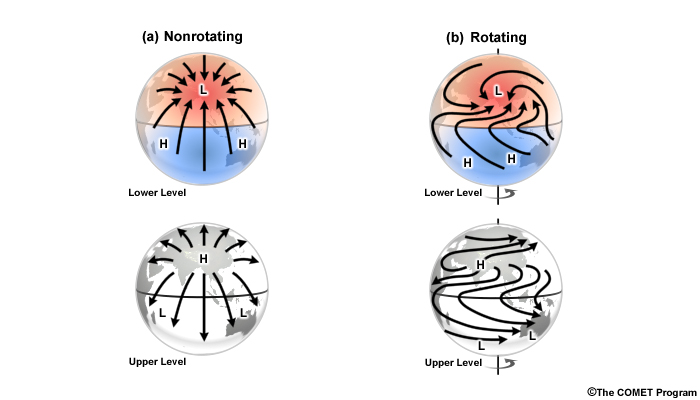
The flow of air follows the basic principles described previously. At the large scale (1000–10,000 km), air flows around low and high pressure areas, creating wave-like patterns. Troughs and ridges in the pressure field are analogous to valleys and mountains in terrain. Air converges into low pressure areas and diverges away from high pressure areas with corresponding vertical motion for mass continuity. Figure 3.3 and the animation linked below illustrate air in motion for low and high pressure areas in the Northern Hemisphere. The direction is opposite in the Southern Hemisphere where the Coriolis force deflection is to the left.
Vertical motion leads to adiabatic temperature change, thus the location of high and low pressures give us information about expected cloudiness and precipitation. Rising motion in low pressure leads to expansion, adiabatic cooling, and condensation while sinking in high pressures leads to adiabatic compression, warming, and dry conditions.
3.1 General Principles of Atmospheric Motion »
Box 3-1 Vorticity
Relative Vorticity
In general terms, vorticity is a measure of the local rotation of the flow; and applies to any environmental fluid flow. In terms of meteorology, flow refers to winds.
Relative vorticity, , is a microscopic measure of the vorticity in a flow.
It is a differential, vector property of the flow.
- Relative vorticity is defined in terms of spatial wind components,
 , as
, as
 (B3-1.1)
- Relative vorticityhas units of s-1; from dimensional analysis of equation (B3-1.1)
- Vorticity is defined as positive in the counterclockwise direction.
- Because horizontal winds are usually larger than the vertical winds at synoptic scales (Section 3.1.2Section 3.1.2), we approximate the relative vorticity as its vertical component, ζ :
 (B3-1.2)
- Horizontal wind components cannot be assumed to be much larger than the vertical wind component in thunderstorms or mesoscale systems.
Earth Vorticity and the Coriolis Parameter, f
The Earth is rotating about its axis at rate (s-1). Since winds are defined relative to the Earth's surface, we express rotation about the Earth's axis, in terms of those same coordinates, as:
 (B3-1.3)
where  is the unit vector pointing north,
  is the unit vector pointing upwards (perpendicular to the surface) and Φ is latitude.
- Changes in latitude affect distance from the Earth’s axis and its vorticity.
- The Coriolis parameter, f, is the vertical component of Earth vorticity (s-1),
 (B3-1.4)
- At the North Pole f=2Ω; at the equator f=0, and at the South Pole f=-2Ω.
- Since the Earth is always rotating in the same direction, why does f change sign when we cross the equator? That is because the Earth vorticity is defined based on our location on the Earth’s surface. Now, think about what the Earth’s rotation looks like from that location. For example, from the North Pole, the sense of the Earth’s rotation is counter-clockwise, which is defined as the positive sense of rotation. From the South Pole, the sense of the Earth’s rotation is clockwise (use a rotating globe to visualize), which is the negative sense of rotation. The sense of cyclonic flow always matches the sense of Earth rotation. Thus, in the Southern Hemisphere, flow with a negative sense of rotation corresponds to cyclonic rotation.
Absolute Vorticity
Absolute vorticity is the vector combination of relative vorticity and Earth vorticity:
 (B3-1.5)
Once again, for synoptic flows we usually consider only the vertical component, η or ζa:
 (B3-1.6)
Potential Vorticity
Potential vorticity (PV) is defined as the absolute vorticity divided by the depth, Δz, of the column of air that is rotating. It has units of m-1s-1. Potential vorticity is conserved in flow that is adiabatic and frictionless, i.e., if there is no diabatic heating or turbulent mixing, potential vorticity remains constant:
 (B3-1.7)
Therefore, for a column of air moving equatorward without a change in depth, its relative vorticity must increase (since f is decreasing) to keep PV constant. If the depth of the column changes because of flow over a mountain, then its absolute vorticity must change, by inducing cyclonic or anticyclonic relative vorticity and/or shifts in latitude (change in f).
Isentropic potential vorticity, P, is the potential vorticity measured between two isentropic surfaces (surfaces of equal potential temperature) and can be defined as
 (B3-1.8)
or written as
where ρ is pressure, θ is the potential temperature, and P is often expressed in potential vorticity units (PVU) where one PVU is 10-6 K kg-1 m2 s-1.
3.1 General Principles of Atmospheric Motion »
3.1.4 Scale Analysis of the Tropics
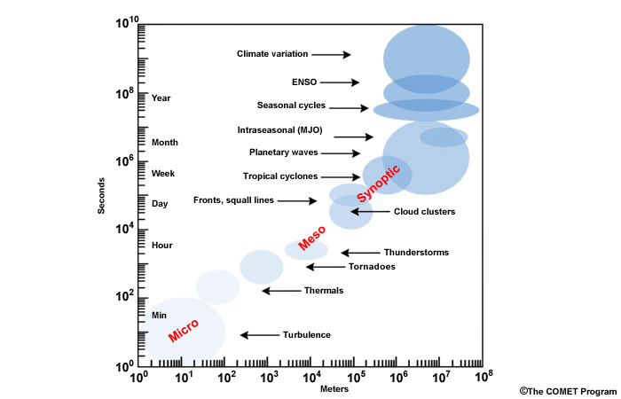
We determine the relative importance of different forces by scaling them according to the basic dimensions of length, mass, time, and temperature. Figure 3.4 shows examples of dynamical processes in the atmosphere classified by their space and time scales (the figure is reproduced from Chapter 1). The basic dimensions are listed in Table 3.1.
| Symbol | Variable | Units |
| U | horizontal velocity | m s-1 |
| W | vertical velocity | m s-1 |
| L | Length | m |
| H | height or depth | m |
| δP/ρ | horizontal pressure fluctuation weighted by density | J kg-1 = m2 s-2, units of geopotential |
| T = L/U | Time | s |
Rossby Number
The Coriolis force goes to zero at the equator therefore geostrophic balance does not apply there. Without geostrophic balance, the winds are not constrained to be parallel to the mass or pressure fields. Therefore, winds at or near the equator are generally divergent and the wind field is easily modified by the mass field.
We can evaluate where to apply the geostrophic assumption by using the dimensionless Rossby number, R0, a ratio of inertial and Coriolis forces, defined as:
 (17)
(17)When winds follow the mass and pressure fields, the Rossby number is small. Table 3.2 shows the variation of R0 with latitude if U~10 m s-1 and L~106 m.
| Latitude, Φ | Coriolis parameter, f = 2ΩsinΦ |
U (m s-1) | L (m) | Rossby Number, R0 U/(f L) |
| 45° | 1.12 x 10⁻⁴ | 10 | 106 | » 0.09 |
| 23.5° | 6.32 x 10⁻⁵ | 10 | 106 | » 0.16 |
| 3.6° | 9.95 x 10⁻⁶ | 10 | 106 | » 1 |
In the midlatitudes, f changes little with latitude. However in the tropics, f is small and its change with latitude is large (see Table 3.2), so we usually assume f ~ Βy, where Β=∂f/∂y. This is called the "Beta-plane assumption" and equatorial flow is referred to as being on a "Β-plane" while midlatitude flow is on an "f-plane".c
Note that R0 changes with the scale of the circulation regardless of latitude.
For the typical scales of mean wind velocity, find the range of L for which geostrophic balance applies in the tropics.
Hint: For the geostrophic assumption to hold, R0 must be small, use R0 = 0.1
Feedback:
You should see that for the geostrophic assumption to hold, large-scale flow in the tropics needs to have sufficiently large L so that R0 is small. In systems with strong winds and small sizes, such as tornadoes, R0 is large and force balance is between the pressure gradient and centripetal forces.
Static Stability and Brunt-VÄisalÄ frequency
A fundamental quantity used to describe vertical motion in the atmosphere and ocean is the Brunt-Väisalä frequency, or buoyancy frequency, N: the frequency at which vertically displaced air parcels will oscillate in a statically-stable fluid. For the atmosphere,
 (18)
(18)where g is the gravitational acceleration (9.8 m s-1), θ is the potential temperature (K), and z is height. For the ocean,  where
where  , the potential density, is dependent on temperature and salinity. N (measured in rad s-1) varies with the stability of the atmosphere or ocean (Table 3.3). For neutral environment, N2 is zero.
| Statically Stable (density decrease with height) | N2 > 0 | Vertically displaced parcel will accelerate towards its initial position, but overshoot, creating an oscillation with frequency, N. |
| Statically Unstable (density increase with height) | N2 < 0 | Vertically displaced parcel will accelerate away from its initial position (leads to convection and overturning) |
The restoring force on displaced parcels is proportional to gravity and the density differences between the initial layer and the layer to which parcels are displaced. The Brunt-Väisalä frequency is the maximum frequency of internal gravity waves between the two layers.
Rossby Radius of Deformation
For fluids that are affected by both gravity and rotation, the Rossby radius of deformation, λR, is the horizontal length scale at which rotation effects become as important as buoyancy effects.
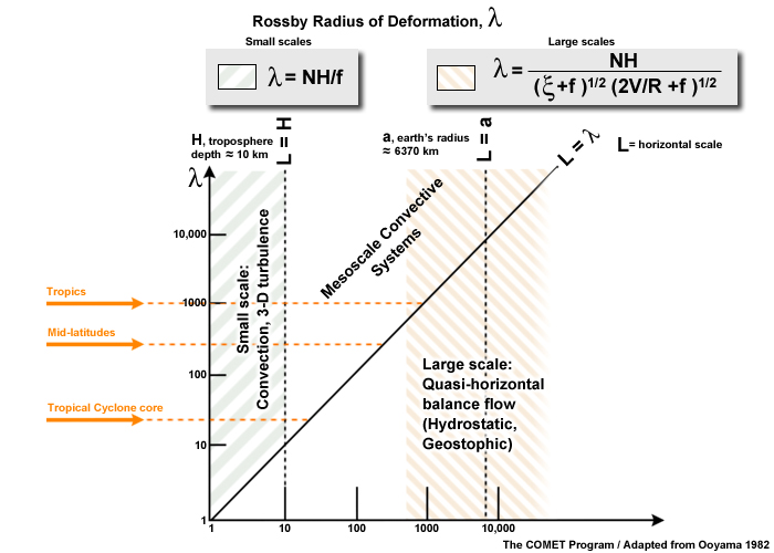
The Rossby radius can be scaled to
 (19)
(19)where N is the Brunt-Väisalä frequency, a measure of static stability, H is the scale height, ζ is the relative vorticity, and η is the absolute vorticity. For typical values of these variables, we can estimate λR.
- In the midlatitudes, λR ≈ 500 km
- At 10°, λR ≈ 2000 km
- At 5°, λR ≈ 10,000 km
- Its value approaches infinity at the equator as f goes to zero.
The practical application of λR is to evaluate whether a pressure or height perturbation feature is dynamically "large" or "small". If it is dynamically "large", it will retain its perturbation characteristics for a considerable period and winds will come into balance with the mass field. If dynamically "small", the feature will decay and the height field will adjust to the remnants of its wind field. Learn more about the Rossby radius of deformation in the COMET module, The Balancing Act of Geostrophic Adjustment, http://www.meted.ucar.edu/nwp/pcu1/d_adjust/.
Scaling of Horizontal Motion
The equation of horizontal motion can be written as
 (20)
(20)and expanded to
 (21)
(21)with basic scales: 
For the midlatitudes
The remaining terms are pressure gradient balanced by the Coriolis force. If Δp/ρL ~ 10-3 then Δp ~ 1000 Pa or 10 hPa for synoptic length scale, L ~ 10-6 m.
For 5°-10° latitude
The remaining terms are 
For balance to be maintained, Δp/ρL ~ 10-4 or Δp ~ 100 Pa or 1 hPa, since L ~ 10-6 m.
For the equatorial zone, 5S°-5N°
The remaining terms are the pressure gradient force balanced by the advection term.
Scaling Vertical Structure at Low Latitudes
The hydrostatic equation can be written as
 (22)
(22)Basic Scales: Since ρ ~ 1 kg m-3, then 
For the tropics, where Δp ~ 100 Pa (see scales above),
Scaling the Thermodynamic Energy Equation
The thermodynamic energy equation (13a) can expressed in terms of the potential temperature, θ, as:
 (23)
(23)and expanded to:
 (23a)
(23a)In the absence of strong diabatic heating, Q/ cp ≤ 1 K day-1 and horizontal temperature advection is balanced by vertical motion of w ~ 0.3 cm s-1.
The horizontal temperature perturbation can be scaled as:
Here, H is a typical scale height (~ 104 m), wind speed, U ~ 10 m s-1, gravitational acceleration, g ~ 10 m s-2, and L is a typical horizontal scale.
- For the tropics, Δθ/θ ~ 10-3
- For the midlatitudes, f ~ 10-4 s-1, L ~ 106 m, so Δθ/θ ~ 10-2
Tropical horizontal temperature gradients are much smaller than in the midlatitudes so horizontal advection cannot balance the large heating observed in moist deep convection. Within precipitating tropical synoptic systems, Q/ cp ~ 5 K day-1, so vertical motion of a few cm s-1 is needed.
c The f- and β-planes are approximations that allow us to think of the surface of the Earth as a tangent plane to the region we are interested in: an f-plane approximates the surface as a cylinder and a β-plane approximates the surface as a cone. In this way, the β-plane varies the distance between the surface and the axis of rotation, so varies the effects of Earth rotation as a parcel moves north or south.
3.1 General Principles of Atmospheric Motion »
3.1.5 The Natural Coordinate System
Since isobaric analysis is less useful for inferring the winds in the tropics, we use kinematic analysis and define motion according to natural coordinate systems instead.
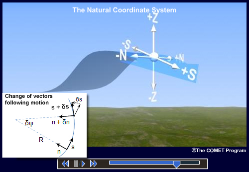
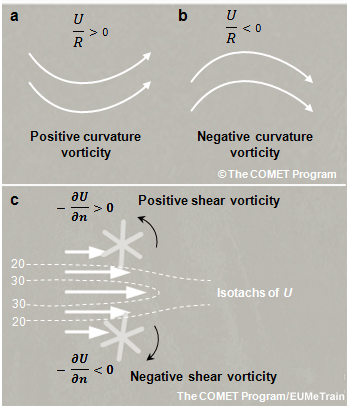
The natural coordinate system describes motion as normal or tangential to the radius of curvature of the flow (Fig. 3.6). Rather than isobars, flow is depicted as streamlines, which represent the instantaneous direction of the wind, and isotachs, the instantaneous wind speed. We can construct natural coordinates with unit vectors n and s, where n is the normal vector and s is the tangential vector. These are related to the vertical unit vector, k, by n = k × s. We can also define an angle Ψ, as the angle that the tangent of the curve makes with a fixed direction, and the radius of curvature of the flow (Fig. 3.6). Note that Ψ is defined as positive in the counterclockwise direction and R > 0 for counterclockwise flow. The continuity equation in natural coordinates is:
 (24)
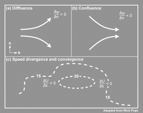
(24)The divergence has two components, the transverse divergence or diffluence, which represents the change in angle with movement across the flow. As streamlines spread out or become diffluent (as in Fig. 3.7a), it is assumed that the air parcels are also diverging from each other. Confluence is shown in Fig. 3.7b. Note, however that regions of diffluence are not always regions of divergence. The continuity equation has a second term, the downstream divergence which measures the change of velocity (Fig. 3.7c). As in (5), we can express the continuity equation in terms of the vertical velocity,
 (25)
(25)
The vorticity equation, defined in Box 3-1Box 3-1, can be written in natural coordinates as
 (26)
(26)where R is the radius of curvature and U is the wind speed. Vorticity in natural coordinates is the sum of the curvature vorticity (Fig. 3.8a,b) and the shear vorticity (Fig. 3.8c).
3.2 General Circulation of the Atmosphere
The general circulation of the atmosphere refers to the mean global flow over a long enough period to remove variations caused by weather systems but short enough to capture seasonal and monthly variability. The major influences on the general circulation of the atmosphere are:
- Differential heating
- Rotation of the planet
- Topography
- Atmospheric and oceanic fluid dynamics
3.2 General Circulation of the Atmosphere »
3.2.1 Historical Evolution of Global Circulation Conceptual Models
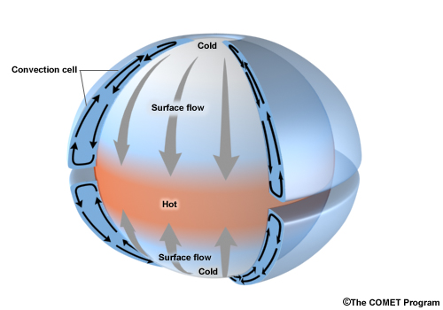
In 1686, Edmund Halley1 provided a theory for the northeast and southeast trade winds. He postulated that the trade winds were the result of cool dense air flowing into a region of hot air, which then rises. In order to preserve equilibrium, the upper air would move from the area of greatest heat to descend and form a circulation cell. He envisioned that the northeast trades wind below would be balanced by a southwesterly flow above and the southeast trades balanced by upper northwestward flow. George Hadley (1735)2 proposed a single axisymmetric cell in each hemisphere that would transport heat from the tropics to the poles. Lord Kelvin (1857, 1892) presented a more complex near surface circulation but retained the single "Hadley cell" circulation aloft.
None of these early theories considered the impact of rotation and the role of angular momentum conservation (Chapter 1, Section 1.8Chapter 1, Section 1.8). A parcel that is displaced across latitudes must conserve its absolute angular momentum. A single parcel moving from the equator to the pole would have to attain an infinitely fast zonal velocity in order to conserve its absolute angular momentum (Table 3.4).
For stationary parcel at equator,
= Ωa2 = 2.96 x 10⁹ m2 s-1
| Latitude | Earth’s Angular Momentum (EAM) × 109 m2 s-1 | Induced Earth-relative wind (m s-1) |
| EQ (0°) | EAMEQ = MEQ = 3.0 | 0 |
| ±30° | EAM30° = 2.2 | 134 |
| ±45° | EAM45° = 1.5 | 327 (~ speed of sound) |
| ±60° | EAM60° = 0.4 | 697 |
| ±90° | EAM90° = 0 | → ∞ !! |
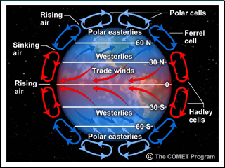
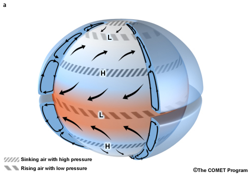
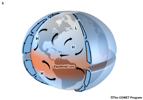
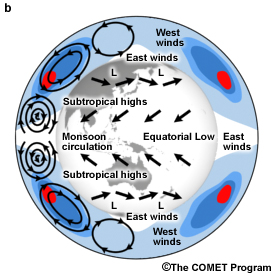
Observations have since confirmed the presence of a Hadley circulation between the equator and subtropics (approximately ±30°). Between 1856 and 1861, William Ferrel proposed that midlatitude circulation cells with westerly winds were caused by air deflected by the Coriolis force.3 In 1921, Wilhelm Bjerknes identified the polar easterlies and proposed that they resulted from a thermally-indirect cell, the Ferrell cell, where balance is maintained by the midlatitude cyclones. Tor Bergeron proposed a three-cell structure and identifies boundaries between air masses in each region. Thus a more complex picture of the general circulation for an aqua planet emerges, with tropical easterly surface winds, midlatitude westerlies, and polar easterlies (Fig. 3.10). When the impact of continents is added, more complex surface patterns develop (Fig. 3.10b). Instead of bands of low and high pressure, areas of high and low pressure form in different regions, e.g., subtropical highs are centered over the ocean.
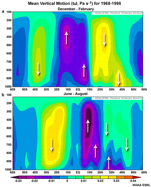
The mean meridional circulation is shown in Fig. 3.11. The tropics are marked by upward motion and the subtropics by sinking motion, forming the Hadley cell. However, the patterns are not mirrored across the equator. The maximum upward motion occurs during the summer over the more continental Northern Hemisphere (Fig. 3.11a). The pattern of rising motion flanked by dual areas of sinking motion occurs only during the southern hemisphere summer. In the north, the continental effects lead to strong upward motion in the lower troposphere during summer and the strong sinking motion during winter.
A theory for the axisymmetric Hadley Cell was first developed for a generic planetary atmosphere by Isaac Held and Arthur Hou (1980).4 Their basic assumptions are a rotating earth with two layers in the atmosphere and motion constrained by the conservation of energy, angular momentum, and mass. See Box 3-2Box 3-2 for more theoretical details.
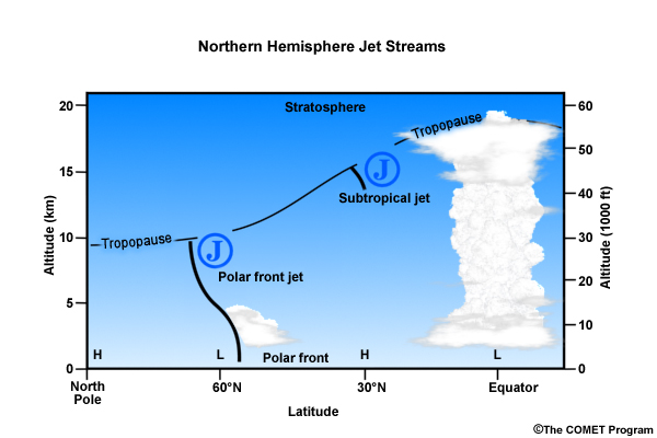
Above the surface, away from friction, winds are generally faster. Near the tropopause, are corridors of very strong winds called jetstreams. Tropical meteorology is most concerned with the Subtropical Jet (STJ, Fig. 3.12) and the Tropical Easterly Jet (TEJ).
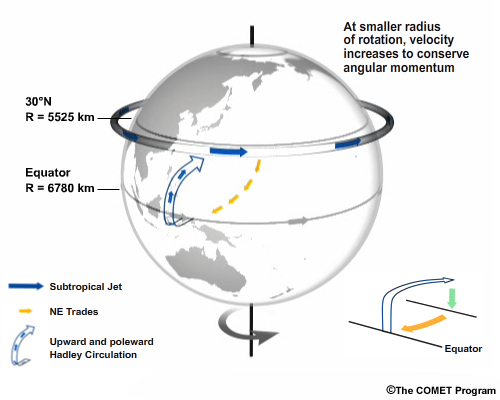
The STJ at about 30° latitude results from the air flowing upward and poleward in the Hadley cell (Fig. 3.12). As air parcels move to a smaller latitude circle, their velocity must increase in order to conserve angular momentum. Note that typical speeds in the STJ are less than calculated using the angular momentum equation (Table 3.4) because large-scale eddies (e.g., cyclones) transport some of the momentum from the Hadley cell to the midlatitudes (Fig. 1.28) and air parcels are slowed by small scale turbulence. Other mechanisms contribute to the variability of the STJ globally, including north-south gradients in mid-tropospheric heating and undulations caused by the Central Asia mountain ranges.
http://www.windows2universe.org/earth/Atmosphere/global_circulation_lsop_video.html
The Polar Jet forms in the region of strongest temperature contrast between cold, polar air and warmer air masses on the equatorward side of the polar front. The Polar Jet is strongest during winter when it can, occasionally, migrate to tropical latitudes. Figure 3.13 shows the relative positions of the westerly jet streams and the mean meridional circulations. As noted in Chapter 1, deep convection places a significant role in the global energy balancedeep convection places a significant role in the global energy balance.5 Carl Gustav Rossby (1941)6 was the first to recognize the explicit role of deep convection in the general circulation (Fig. 3.13a). Organized, deep convection often occurs where divergence in the upper-level jet streams is associated with a low-level wind maximum known as a low-level jet. We will learn more about low-level jets in the tropics in Focus Section 2Focus Section 2.
3.2 General Circulation of the Atmosphere »
Box 3-2 Axisymmetric Hadley Cell: Theories and Assumptions
The Hadley cell is vital to the poleward transportation of energyenergy and angular momentumangular momentum. The latitudinal extent of Hadley cells is related to the static stabilitystatic stability in the subtropics (which forms the outer boundary of the Hadley cell), the differential diabatic heating poleward from the equator, rotation of the Earth, and conservation of angular momentum. Most of what we understand about the Hadley cell comes from simple theories. According to one theory,4 the zonal wind in the upper branch of the Hadley cell is controlled by conservation of angular momentum and the Hadley cell is a closed system for energy transfer, so that the diabatic heating in the regions of ascent is balanced by diabatic cooling in regions of descent. The mathematical expression of this theory can be simplified7 by using a β-plane approximation to transform the problem to rectangular coordinates. The poleward extent of the Hadley cells can then be derived as follows:
Geometric assumptions
- Scale Height, H, is much smaller than Earth’s radius, a.
H << a, a = 6.37 x 10⁶ m
- 2 layers in the vertical
- Earth’s rotation is constant at Ω = 7.292 x 10⁻⁵ rad s-1
- That at small latitudinal angle, Φ,
sin(Φ) ≈ Φ, cos(Φ) ≈ 1
y = a Φ, so YC = a ΦC
Using the small angle approximation for a β-plane gives
f = βy β=2Ω cosΦ /a (B3-2.1)
And for an equatorial β-plane this reduces to
f = 2Ω y/a β= 2Ω/a (B3-2.2)
Balance assumptions (dynamic constraints)
- Steady state

- Axisymmetric

- Hydrostatic
 (B3-2.3)
 - Thermal wind balance
 (B3-2.4)
- Conservation of absolute angular momentum
M(Φ1) = M(Φ2), where M= (Ωa cos(Φ) + u) a cos(Φ) (B3-2.5)
Thermal Forcing (thermodynamic constraints)
- θE(Φ) is the equilibrium potential temperature distribution that results from the distribution of incoming solar radiation (in radiative equilibrium).
- Dynamical response to this thermal forcing redistributes temperatures to θ0(Φ) ≠ θE(Φ)
- Thermal forcing towards θE(Φ) due to solar radiation can be written as
 (B3-2.6)
where τE is the relaxation time scale over which θE(Φ) would return to θE(Φ) if the other forcings (motion) ceased.
The result is an equation for the difference in the mean equatorial potential temperatures, θE, in radiative equilibrium and momentum balance
 (B3-2.7)
…and a second equation for the latitudinal extent of the Hadley cell, ΦH,
 (B3-2.8)
where Hτ is the height of the tropical tropopause, θ0 is global mean temperature, Δθ is the equator-to-pole surface potential temperature difference in radiative equilibrium—the primary thermodynamic factor in this theory.
Another theory assigns Hadley cell width as the latitude to which the angular momentum conservation continues until the vertical shear leads to baroclinic instability. That latitude is defined as:
 (B3-2.9)
where ΦH is the Hadley cell latitude, He is the tropopause height at that latitude, N is the Brunt-Väisalä frequency. Here the major thermodynamic factor is the dry static stability of the subtropics.
Why should we care about changes in the Hadley cell poleward extent? Satellite observations, radiosonde data, and global reanalysis indicate that the Hadley cell has widened by about 2 to 4 degrees latitude since 1979.8,9,10 The location of its boundaries, the subtropical dry zones, deserts, and jet streams have shifted poleward. If this trend continues it could have important societal impact, such as drier climates where people are used to established rainfall patterns or ecological changes in plants, insects, or animals.
3.2 General Circulation of the Atmosphere »
3.2.2 A Road Map to the Tropics and Subtropics
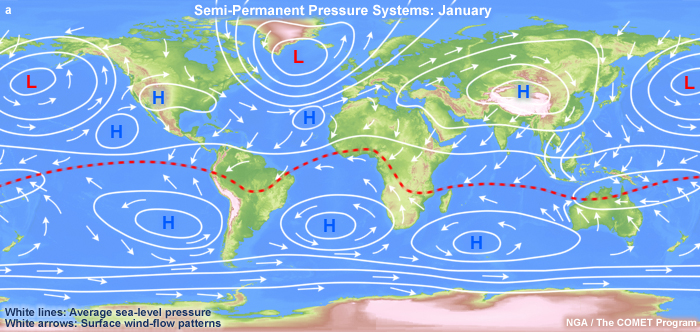
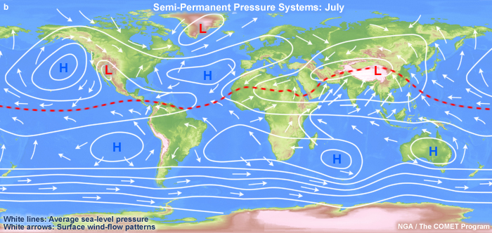
The general circulation of the tropics is dominated by quasi-stationary circulations that vary little in time and monsoonal circulations that are seasonally reversing (Section 3.4Section 3.4). At the center is the equatorial trough, the zone of low pressure that forms in response to net heating and rising air (Fig. 3.14). During the boreal summer (July), the most prominent low pressure centers are the thermal lows over India, the Sahara Heat Low over Africa, and the Sonora Low over North America (Fig. 3.14b). The austral summer (January) has prominent lows over the subtropics of South America, southern Africa, and Australia-Indonesia (Fig. 3.14a). The subtropics are dominated by the Pacific-Hawaiian High and Bermuda-Azores High of the Northern Hemisphere and their counterparts over the Southern Hemisphere all of which have mean pressure of about 1020 hPa but are strongest during their respective summers. Note the more zonal nature and less dramatic seasonal changes in the southern hemispheric because it has less land. The trade winds, the lowest branch of the Hadley cells, play a significant role in shaping the weather and ocean interactions in the tropics. They are fairly persistent, steady, and have average speeds of 4-7 m s-1, with stronger speeds in the winter. Clouds in the trade wind regime increase in altitude towards the west (Fig. 1.18b) and towards the equator (Chapter 5, Section 5.2.2.3Chapter 5, Section 5.2.2.3, Fig 5.16). Trade winds are affected by interannual oscillations such as the El Niño Southern Oscillation (ENSO)El Niño Southern Oscillation (ENSO).
The meridional and zonal variation in the locations of the pressure centers is driven by atmospheric response to non-uniform surface properties. For instance, the mean location of the equatorial trough and the ITCZ is north of the equator, creating a "meteorological equator" near 5°N. The southern ITCZ is usually a springtime feature in the east Pacific and in the western Atlantic only in the summer. However, recent QuikSCAT satellite wind data have confirmed the existence of a southern ITCZ across the Atlantic and Pacific. What is controlling the meridional variation in the ITCZ location? Several explanations have been offered including: cooling of the equatorial Pacific by Ekman pumping, the availability of moisture, strong gradients or maxima of SST, the location of continents, the Andes Mountains. A special box section discusses some of the theories for the ITCZ location over the tropical Eastern Pacificspecial box section discusses some of the theories for the ITCZ location over the tropical Eastern Pacific.
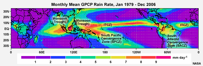
In between the tropics and the midlatitudes are the convergence zones of the South Pacific (SPCZ) and South Atlantic (SACZ) which are associated with annual rainfall maxima (Fig. 9. 31). An intermittent convergence zone also exists over southeastern Africa and the Indian Ocean. These convergence zones are the corridors of poleward moving tropical and subtropical cyclones and their location is influenced by the SST gradients and the variability of the subtropical highs.
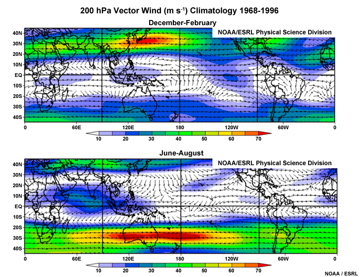
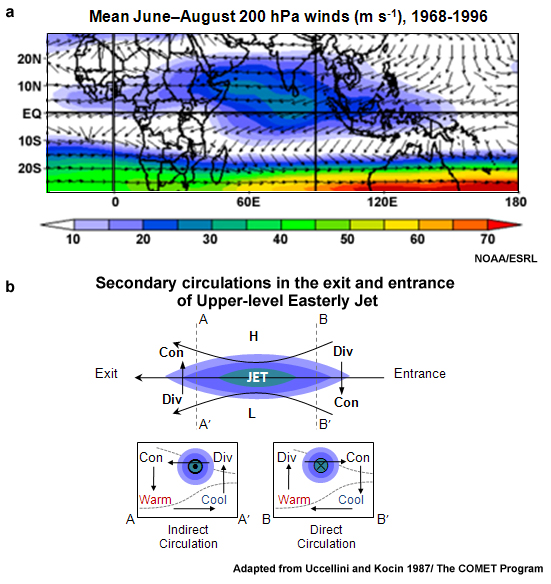
Upper tropospheric winds (Fig. 3.15) are nearly zonal compared with the more complex surface patterns. Yet even at such high altitudes, the continental effect is evident in the undulations near the coasts and variation in wind speeds. Note the strong jets emanating from the east coasts of Asia and North America. The pattern is more zonal and jets are stronger over the Southern Hemisphere because of the smaller land mass. The STJ exists all year in the Southern Hemisphere but disappears in the Northern Hemisphere in the summer, due to reduction in the north-south temperature gradient. While not as strong as the westerly jet streams, maxima in the tropical upper-tropospheric easterlies occur during the summer (Fig. 3.15b). These maxima reflect the Tropical Easterly Jet (TEJ) found near 100-150 hPa.11 The TEJ forms in response to meridional heating surplus over tropical land masses, which helps to establish upper level high pressure and strong easterlies, with maximum speed of 40-50 m s-1, over central and southern India.
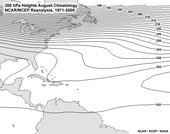
Tropical Upper Tropospheric Troughs (TUTTs)12 are semi-permanent features found over the tropical oceans during summertime (e.g., Fig. 3.16). They are associated with enhanced convection in the tropics and occasionally with tropical cyclone genesis. The strongest TUTTs are found in the North Pacific, North Atlantic, Caribbean, and Gulf of Mexico. The east Pacific region is the most prominent in the Southern Hemisphere; weaker ones are found over Australia, South America, and occasionally, Africa. TUTTs are described in more detail in separate chapter sections on synoptic weather systems and synoptic weather analysissynoptic weather analysis.
3.2 General Circulation of the Atmosphere »
3.2.3 Comparing the Tropics and Midlatitudes
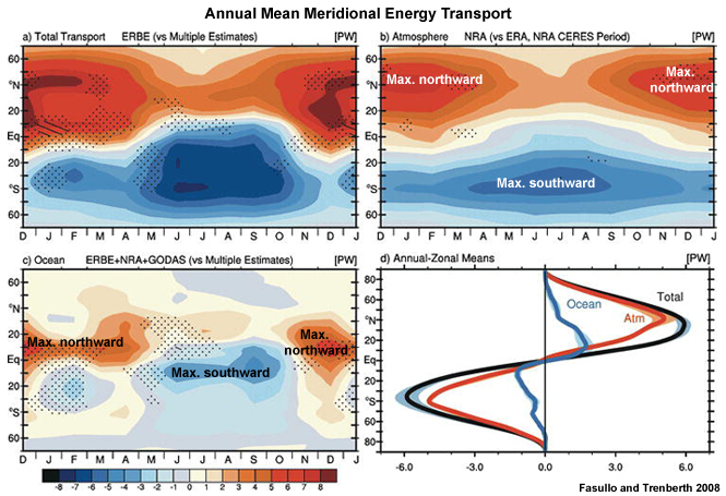
During the annual solar cycle, the tropics receive heating all year while the midlatitudes receive their maximum heating during their respective solstices. The tropics have a surplus of radiation heating while the midlatitudes have a deficit (Fig. 1.1). In the tropics, surplus heat is transported poleward by ocean currents and the Hadley cells, with maximum transport between 10 and 15 degrees latitude (Fig. 1.12d), while transient eddies transport most heat in the midlatitudes (Section 1.4.2Section 1.4). The tropics are cooler than expected from solar radiation.
The tropical atmosphere is in near thermal inertia because of the warm ocean surface currents and moist planetary boundary layer. The vertical wind shear is much weaker in the tropics; about 20% of midlatitude shear on average. For the same scales of motion and in the absence of strong convection, the vertical velocity in equatorial regions is much smaller than the vertical velocity in the midlatitudes.
The large-scale midlatitude atmosphere is noted for being baroclinic while barotropic conditions are usually found in the tropics for these scales. Being baroclinic means that density is a function of pressure and temperature or ρ = ρ (p,T), i.e., the density and temperature vary along a pressure surface. Streamlines and isotherms cross each other. By comparison, in a barotropic fluid, the density is a function of pressure only, ρ = ρ (p); i.e., an isobaric surface is the same as a constant density surface and the temperature and density fields are parallel. Streamlines and isotherms are parallel to each other. Midlatitude eddy motions, such as midlatitude cyclones, result from baroclinic instability. The atmosphere tries to reduce the imbalance created by strong gradients of temperature and density and return to zonal flow. Midlatitude cyclones are cold core systems whose cyclone strength increases with height. In contrast, tropical cyclones are warm core systems without fronts and whose cyclonic circulation weakens then reverses with height.
Tropical circulations, such as the semi-permanent pressure systems, the longitudinally dependent components of the general circulation, and the monsoons, together account for the low frequency variability13 of the tropics compared with the higher frequency variability of the midlatitude general circulations.
3.2 General Circulation of the Atmosphere »
3.2.4. Stratospheric Circulations
3.2 General Circulation of the Atmosphere »
3.2.4. Stratospheric Circulations »
3.2.4.1 Brewer-Dobson Circulation
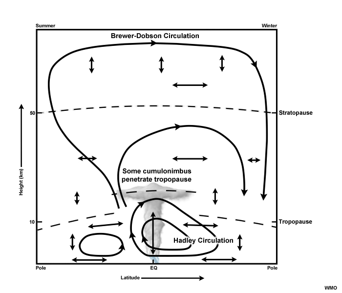
The tropopause is highest and coldest in the tropics at 16-17 km (Fig. 1.16). Brewer (1949) examined humidity measurements from radiosondes and theorized that the low levels of humidity in the stratosphere indicated that air entered the stratosphere through the cold point tropopause (CPT) in the tropics. The general circulation in the stratosphere, known as the Brewer-Dobson circulation,15,16 has air, dried by condensation, moving from the tropics to the poles leading to the transport and accumulation of ozone at the winter pole (Fig. 3.17). The Brewer-Dobson circulation is driven by buoyancy waves in the atmosphere which form when air flows over high mountains and tall thunderstorms. The waves propagate upwards, become amplified, and break in the middle stratosphere, which creates a drag on the existing flow. Like the tropospheric circulations, the stratospheric circulation is also partly driven by imbalances in radiation. The stratosphere becomes cooler at the dark, winter pole leading to a pressure gradient force and flow towards the winter pole.
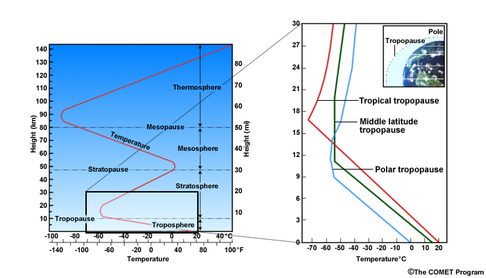
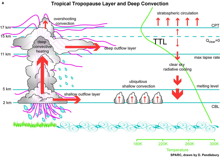
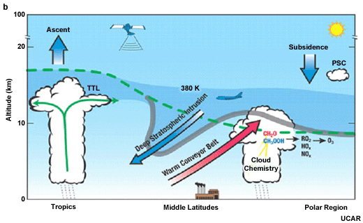
The Tropical Tropopause Layer (TTL) is the transition between the convectively-dominated troposphere and the stratosphere, extending from lapse rate minimum level at 10-12 km to the cold point at 16-17 km (Fig. 3.18a).17 The TTL is relatively undisturbed as the influence of convection decreases with height. It is subject to prolonged chemical processing of air parcels. Active deep convection has a greater impact on stratospheric intrusion than weaker (non-active) regions.17 The cold point tropopause is highest in January–March (northern winter) and lowest in June–August (northern summer). The trend since 1978 has been rising of the cold point level by 20 m per decade, cooling by 0.5 K per decade, and decrease in pressure by 0.5 hPa per decade.9 Studies of the TTL continue in order to understand the ways that air enters the stratosphere such as through convection up to the cold point tropopause, slow radiative lifting, moistening/dehydration mainly as convective phenomenon, or cirrus formation.
3.2 General Circulation of the Atmosphere »
3.2.4. Stratospheric Circulations »
3.2.4.2 Quasi-Biennial Oscillation (QBO)
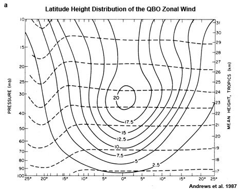
The equatorial stratosphere is also marked by a quasi-biennial oscillation or QBO of the zonal wind; winds shift from easterlies to westerlies. The oscillations are symmetric about the equator (Fig. 3.19a) and originate at about 40 km (near 20 hPa) and propagate downwards (Fig. 3.19b). The QBO period is 22-34 months and its maximum amplitude is 20-30 m s-1 (Fig. 3.19b). The QBO was discovered in 1960 by Reed19 and independently in 1961 by Veryard and Ebdon.20
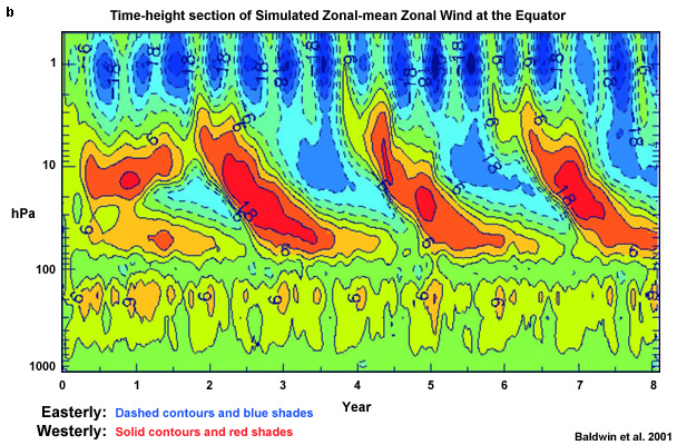
The easterly and westerly modes are asymmetric. The switch from easterly to westerly propagates downward faster than the west to east switch. Westerly accelerations appear first at the equator and spread to higher latitudes, while the easterly accelerations are more uniform in latitude. Westerly accelerations are more intense. More detailed information about the QBO, its evolution, structure, and theories for its formation, is presented in the chapter on tropical variabilitychapter on tropical variability.
3.3 Ocean Circulation
3.3 Ocean Circulation »
3.3.1 Global Upper and Deep Ocean Circulation
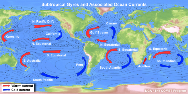
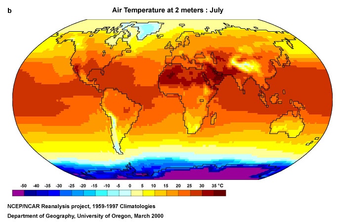
The ocean currents develop in response to wind stress. The semi-permanent surface wind circulations (the subtropical highs and trade winds shown in Fig. 3.14) help to drive the ocean gyres (Fig. 3.20). Currents are defined by temperature; cool currents bringing cool water from the poles and warm current bringing warm waters from the equator to the poles. The prevailing ocean currents are major controls of surface temperature leading to cooler eastern tropical oceans and adjacent coastal areas and warmer western tropical oceans and east coasts (Fig. 1.23, Chapter 1, Focus Section 2Chapter 1, Focus Section 2).
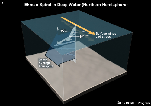
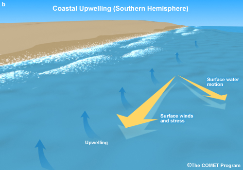
The direction of the currents is not an exact match of the wind. The surface stress decreases with depth leading to decreasing current speed and a spiraling of the water current vector (the Ekman spiral)23 shown in Fig. 3.21a. The mean surface current is about 45 degrees to the right of the wind in the Northern Hemisphere and to the left of the wind in the Southern Hemisphere; because like the air, the water is affected by Coriolis deflection. As surface water is removed, it is replaced with deep water, a process called upwelling (Fig. 3.21b).
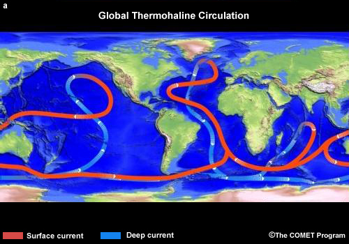
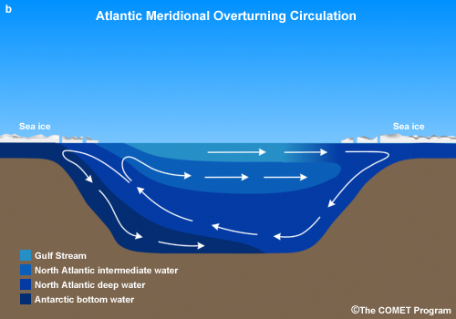
Ocean circulations are also driven by differences in temperature and salinity (Fig. 1.10b) as temperature and salinity gradients lead to density variations and vertical circulations known as the thermohaline circulations. Cold water is denser than warm water and salty water is denser than fresh water so colder or saltier water tends to sink relative to warmer or fresher water. For example, in the north Atlantic, water sinks as the Gulf Stream cools and freezing increases the salinity of the upper ocean. The global ocean conveyor belt (Fig. 3.22a) is the resultant mean ocean transport of surface and deep ocean waters.
Smaller scale ocean waves and vortices, collectively referred to as "eddies" are critical to regional ocean circulations. As noted in Chapter 1, because of its larger heat capacity, the oceans are vital to storage and release of heat and transportation of heat from the tropics to the poles (Section 1.4.2Section 1.4.2).
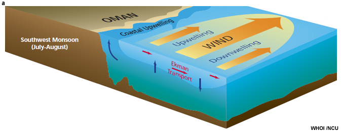
Ocean circulations are also affected by interactions with bottom topography and lateral boundaries. Figure 3.23a illustrates the response of the upper ocean to the strong southwesterlies of the Indian monsoon and the boundary of the Arabian Peninsula. The surface winds drives water to its right (red arrows). The movement of waters away from the coast leads to upwelling of cool water. Variations in the horizontal wind lead to differences in the Ekman transport, which leads to divergence of surface water and downwelling offshore (downward blue arrows) and upwelling on the onshore side of the wind maximum.

3.3 Ocean Circulation »
3.3.2. Ocean Dynamics
Large-scale ocean circulations obey the same fluid dynamics as the atmosphere (Section 3.1Section 3.1). Except for the assumption of a constant reference density, the horizontal equations of motion are similar:
 (28)
(28) (29)
(29)where u and v are the zonal and meridional components of motion; p is pressure ; f is the Coriolis parameter, and F represents frictional terms.
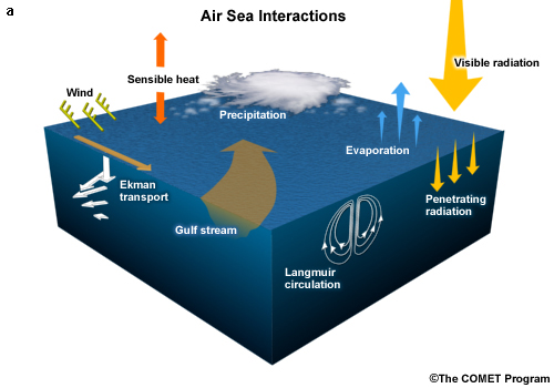
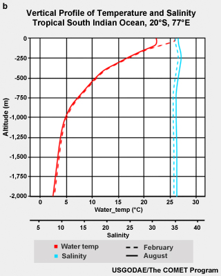
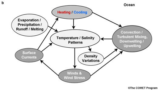
Vertical motions are driven by density variations caused by temperature and salinity gradients. Those gradients can be changed by evaporation, precipitation, freshening, or melting of sea ice and other processes (Fig. 3.24a). The upper ocean is much more responsive to radiative heat changes than deeper in the ocean as illustrated in Fig. 3.24b. Note the large difference between the summer and winter temperature near the ocean surface compared with similarity of temperature at lower depths (red line in Fig. 3.24b). The thermocline can be identified in Fig. 3.24b as the layer separating the near-surface warm, mixed layer from the deeper cool waters of oceans and lakes. In the ocean, the (same) thermocline also separates the fresher water near the surface from the saltier water below (note the tilt in the salinity profiles near the surface in Fig. 3.24b).
3.4 The Response to Equatorial Heating
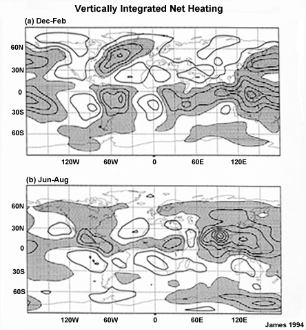
The general circulation has been formulated as a response to surplus heating in the tropics. As was noted in Chapter 1, while the incoming solar radiation is zonally symmetric, the net heating is not. The net heating depends on many factors such as surface properties and the distribution of clouds. Figure 3.25 shows that the vertically integrated net heating is maximized over the continents and over warm ocean currents. The magnitude of the maxima is considerably greater than the magnitude of the minima.
What then is the nature of the dynamical response to net heating? The dynamical response of the atmosphere to imposed heating at the equator was modeled by several scientists, most notably, Matsuno (1966)25 and Gill (1980).26 They found significant zonally asymmetric components to the tropical circulation. Using the Shallow Water Equations, one formulation of the principles of motion and continuity described in Section 3.1Section 3.1, they calculated wave solutions that were later confirmed by observations.
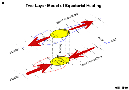
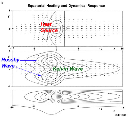
The solutions to their formulation were waves that propagated zonally along the equator and extended vertically to the upper troposphere and lower stratosphere (Fig. 3.26a). The influence of heating extends farther to the east and then to the west but the amplitude of the response is greater to the west (Fig. 3.26b). The solution is confined much closer to the equator on the east that on the west. Some of these equatorially-trapped waves propagated eastward and others westward. The schematic in Fig. 3.26b shows the eastward-moving Kelvin wave and westward-moving Rossby waves that are generated in response to a heating source on the equator. These waves are sometimes coupled with strong convection, especially over the Indian and western Pacific oceans, where they can occasionally lead to tropical cyclone genesis.
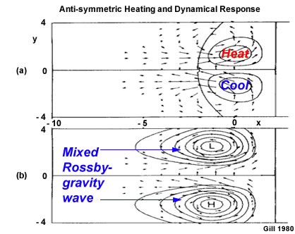
With the heat source distributed anti-symmetrically relative to the equator (Fig. 3.27a), the result is opposing high and low pressure across the equator (Fig. 3.27b). A long planetary wave develops to the west of the heating source. Rising motion and cyclone circulation are associated with the surplus heating and corresponding subsidence with the anticyclone. There is little response to the east. The dominant response is an anti-symmetric equatorial wave termed a mixed Rossby-gravity wave (Fig. 3.27b). We will explore more about equatorial waves in the chapter on tropical variabilityexplore more about equatorial waves in the chapter on tropical variability.
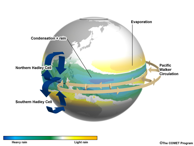
Tropical circulations result from a combination of symmetric and anti-symmetric heating. A result of the anti-symmetric heating is the Hadley cell in July (blue arrows in Fig. 3.28), which has a rising branch over the Northern Hemisphere surplus heating region and a sinking branch over the Southern Hemisphere cooling region. One example of the response to symmetric heating component is the Pacific branch of the Walker Circulation, an east-west circulation, which has rising motion associated with the surplus heating over the warm western Pacific (light brown arrows in Fig. 3.28). The largest of the circulation cells oriented along the equator extends across the Pacific Ocean and was named the "Walker Circulation", in honor of Sir Gilbert Walker, who recognized its existence from observations of pressure oscillations between Darwin in Australia and Tahiti in the Pacific. The oscillation of pressure between Darwin and Tahiti has been codified as a Southern Oscillation Index (SOI). The Walker Circulation now refers to the global mean east-west circulation which consists of large regions of rising motion over the Maritime Continent, tropical South America, and tropical Africa with subsidence in between.
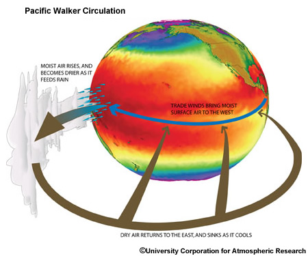
The dominant variability of the Walker Circulation is the El Niño-Southern Oscillation (ENSO), a coupled atmospheric ocean phenomenon with a 2-7 year cyclecoupled atmospheric ocean phenomenon with a 2-7 year cycle. The normal Walker circulation is accompanied by cold upwelling in the east and warm SSTs in the west. During an El Niño, the east and central Pacific become anomalously warm and the west anomalously cooler and the atmospheric circulations, the Southern Oscillation, shift in response to the surface warming. The perturbation of the Walker circulation causes major shifts in atmospheric circulations, rainfall patterns, and seasonal climate across the globe. The cool extreme of ENSO is termed La Niña.
3.5 Monsoons
3.5 Monsoons »
3.5.1 Defining the Monsoon
The monsoon is important because most of the world's population live in monsoon regions. Many of these societies rely on rain-fed agriculture for their food, so the prediction of the amount, timing, and location of monsoon rains is crucial.
The word monsoon comes from the Arabian word 'mausim' meaning 'season' and was first used to refer to seasonal reversal of the prevailing surfaces winds over southern Asia and the Indian Ocean. Different precipitation regimes accompanied the seasonal wind shifts; rains with onshore flow in the summer and a dry winter season with offshore flow. This simple picture has since been found to be a complex system whose onset, intensity, and break periods are among the most challenging forecast problems.
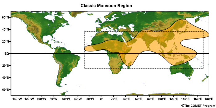
The classical criteria for a monsoon as specified by Ramage (1971)27 are:
- Prevailing wind shifts 120° between January and July
- Average frequency of prevailing wind > 40%
- Speed of mean wind exceeds 3 m s-1
- Pressure patterns satisfy a steadiness criterion
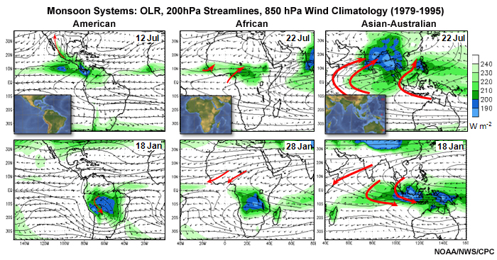
The monsoon regions for which these criteria apply are shown in Fig. 3.29. The Indian monsoon matches these criteria. In the decades since, the monsoon regions have been expanded (Fig. 3.30). The global monsoon systems now include regions of the Americas whose summer time precipitation and wind characteristics are similar to the Indian monsoons. However, as the left panels in Fig. 3.30 show, those regions do not have a winter equivalent so do not match the classical criteria for a monsoon.
3.5 Monsoons »
3.5.2 A Conceptual Model of Monsoon Evolution
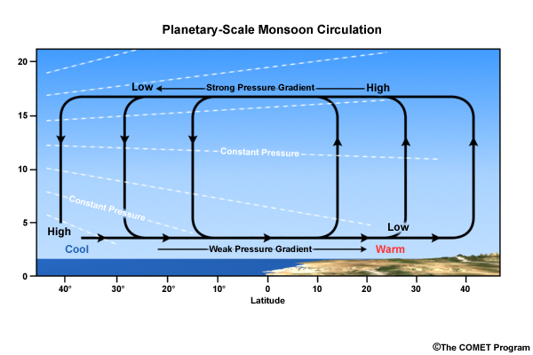
What causes the monsoon? This has been a question since time immemorial. A conceptual model presented by Webster (1987)28 builds on the theories of Halley (1686)1 and Hadley (1735)2 and adds moisture feedback through convection. Figure 3.31 illustrates the conceptual model of the planetary monsoon as a moist sea-breeze modified by the Coriolis Effect. However, the importance of the hot land-cool ocean contrast can be questioned because the land surface temperatures actually decrease during the monsoon (Focus Section 1.2Focus Section 1.2, Box 1-2Box 1-2). Decades of satellite imagery have shown that the south Asian monsoon is not just a local land-seabreeze. Rather it is part of the planetary-scale rain band (associated with the equatorial trough) that is present over all of the warm tropical oceans and differs only in its amplitude in the monsoon regions.29,30 So the planetary-scale monsoon can be considered to have these fundamental mechanisms:
- The seasonal oscillation of solar heating with net heating in the summer hemisphere, which leads to migration of the equatorial trough and the tropical convergence zones
- The differential heating between the land and ocean and the resulting pressure gradient (Halley 1686)
- The swirl introduced to the winds by the rotation of the Earth (Hadley 1735)
- Moisture processes and convection
While the monsoon rains over land are of primary societal concern, many cloud systems that bring rain to the continent are born over the warm oceans.31 For example, during the onset phase of the south Asian monsoon, the oceanic rain band moves northward into the continent. While the global monsoon system responds to net heating on planetary scales, the evolution of the regional monsoons depends on the distribution of land and ocean as well as SST gradients and topography.
Conceptually, the global-scale summer monsoon is a first response to the positive net radiation in the summer hemisphere as the surface responds to the seasonal oscillation of solar heating. The evolution of the regional monsoons depends on the distribution of land and ocean, SST gradients, and net ocean heat transport. Differences in the heat capacity of the land and ocean result in large temperature gradients between the land and ocean surfaces. Horizontal temperature gradients lead to upper level pressure gradients and horizontal pressure gradients and a transverse circulation. Over land, the only way to transport heat downward is through molecular diffusion with little storage while mixing in the ocean allows heat to be transported downward and stored.28
The circulation is not directly from ocean to land because the Earth's rotation causes the Coriolis deflection and affects where the winds and ocean currents form and how intense they become. Finally, the moist processes within clouds affect the vertical velocity and the radiative effects of the clouds in turn affect the differential heating between cloudy and non-cloudy areas.

The major features of the South Asian summer monsoon are the monsoon low, low-level onshore and cross-equatorial flow, Mascarene High, updrafts in moist convection, upper-level high, and TEJ (Fig. 3.32).32 The TEJ is the upper-level venting system for the strong southwest monsoon (Fig. 3.33). These regional responses are coupled with the planetary scale general circulation as illustrated in Fig. 3.32.
3.5 Monsoons »
3.5.3 Evolution of the Asian Monsoon System
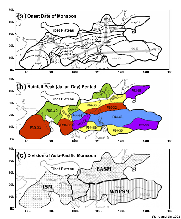
The Asian monsoon is regionally varied. The earliest onset is over the southern Bay of Bengal in late April, over the Indo-Chinese peninsula and south India in early May, and then it progresses north and northwestward into the continent reaching Japan by late June to July (Fig. 3.34a). By the end of the peak season over Japan, the monsoon is already retreating over India (Fig. 3.34b). Given the regional evolution, the Asian monsoon can be divided into two separate but interactive monsoon sub-systems: the Indian Summer Monsoon or South Asian monsoon and the East Asian monsoon (Fig. 3.34).33 The latter can be sub-divided into the East Asian and Western North Pacific monsoon.
Animation of Asian-Australian monsoons (OLR, 850 hPa winds, 200hPa streamlines),
http://www.cpc.ncep.noaa.gov/products/Global_Monsoons/Asian_Monsoons/Asian_Monsoons.shtml
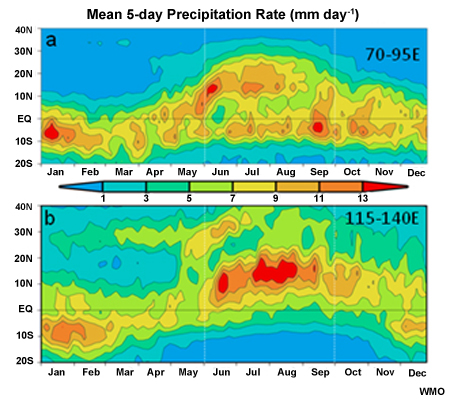
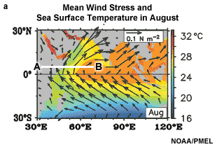
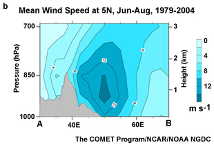
The South Asian monsoon is the northern branch of the seasonal migration of the east-west oriented precipitation belt (the ITCZ) (Fig. 3.35). The precipitation belt migrates from the southern to the Northern Hemisphere in the boreal summer and vice versa in the boreal winter (austral summer).36 The northern most extent of the tropical rain belt in the South Asian monsoon is about 20°N and it retreats to about 5°S during the winter. Two locations are favorable for the rain band: over the heated subcontinent (in keeping with the early theories) and the warm eastern equatorial Indian Ocean. This oceanic cloud band can aid or suppress the main monsoon rains. If the oceanic precipitation is intense, it leads to subsidence over land.36 Strong surface temperature gradients (Fig. 3.36a) lead to large-scale pressure gradients and cross-equatorial winds between the south and north Indian Ocean. Over India, the mean surface pressure at 20°N ranges from 1016 hPa in the winter to 1002 hPa at the peak of the summer monsoon.37 The Somali Jet is the result of the strong temperature and pressure gradients and channeling of the cross-equatorial flow by the East African Mountains (Fig. 3.36b).
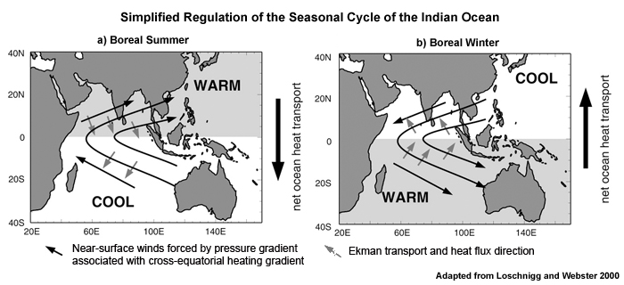
The annual monsoon cycle is regulated by heat transported across the equator by the atmosphere and the ocean. Oceanic heat is transported southward during the summer monsoon and northward during the winter monsoon over the Indian Ocean (Fig. 3.37). The southward movement of heat tends to cool the South Indian Ocean while the northward transport warms the North Indian Ocean southward heat flux in the summer tends to cool the North Indian Ocean. The coupled ocean-atmosphere interaction reduces the SST gradients and imposes a strong negative feedback on the system thereby regulating the seasonal extremes of the monsoon. While the north-south gradient dominates, an east-west SST gradient is also present (Fig. 3.36a).
The annual cycles of the monsoons over India and East Asia are different primarily because the atmospheric response to heating is affected by land-ocean distribution and topography. The strong north-south gradient between the warm land and the cool ocean, enhanced by the heating of the elevated Tibetan Plateau, creates a strong monsoon over India. Over East Asia, the situation is more complex. The forcing comes from both the north-south gradients between cool Australia and warm western north Pacific and east-west gradient between the heated Asian landmass and the cooler Pacific. The result is a weaker monsoon circulation and bands of precipitation along the tropical monsoon circulation and subtropical frontal zones, which we will now examine in more detail.
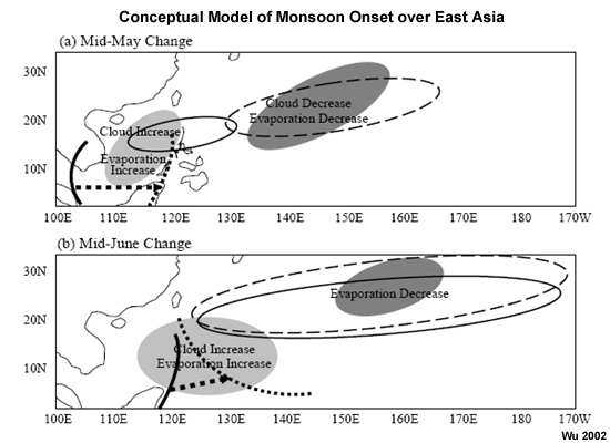
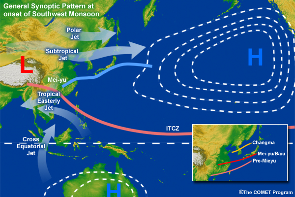
For the East Asian monsoon, the area of clouds and evaporation increases during mid-June relative to the mid-May pattern and the longitudinal extent of the southwesterly winds shifts east into the Pacific (Fig. 3.38a). The Pacific High shifts east and north after the mid-May onset, expands, and strengthens (Fig. 3.38a). A large, thermal trough replaces the subtropical ridge over the continent. Air flows into the equatorial trough, which leads to cloudiness in the ITCZ. The Monsoon Trough extends northwestward from the equatorial trough into the continent. Other features are similar to the South Asian monsoon, the TEJ in the upper troposphere and the cross-equatorial flow at low-levels. To the north at the upper levels is a weakened Subtropical High (Fig. 3.38).
Mei-yu/Baiu Front
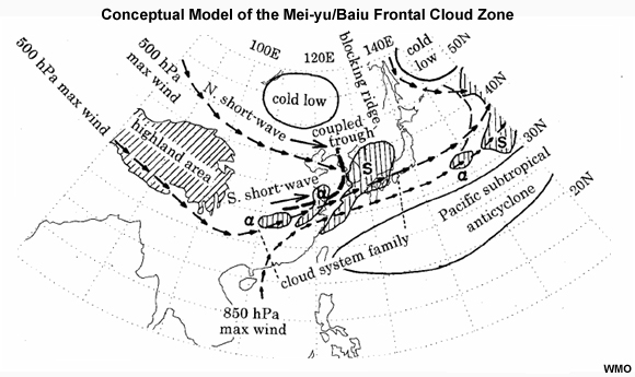
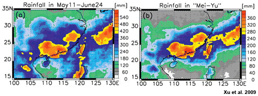
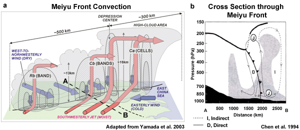
A prominent, signature feature of the East Asian spring and early summer is the Mei-Yu/Baiu front, a semi-permanent, quasi-stationary, weak frontal zone that extends from eastern China east-northeastward into the Pacific (Fig. 3.39). To the north, in Japan, the frontal zone is called the Baiu front, and, in Korea, the Changma front (their relative locations are shown in the inset map on Fig. 3.39a). The Mei-yu and Baiu fronts begin in mid May and continue through early to mid summer while shifting northward. The Mei-yu front is the focal point for persistent heavy precipitation produced by mesoscale convective systems (MCSs) that form and track eastward along the front (Fig. 3.40). Instability, strong rising motion, and persistent deep convection are associated with a low-level jet that brings warm moist air from the South China and Bay of Bengal, low-level warm-air advection, and upper-level divergence, strongest in the right forward quadrant of the Subtropical Jet (Fig. 3.41). Most of the heavy rain is south and east of the front, an area of high relative humidity (Fig. 3.41b). The Baiu front is more typically midlatitude in structure. Weak cyclonic disturbances move along the Baiu front at 3-day intervals. They bring stratus, fog, and light rain to northern edge of the front and thunderstorms and heavy rain along and immediately south of the front.
West Pacific Monsoon trough
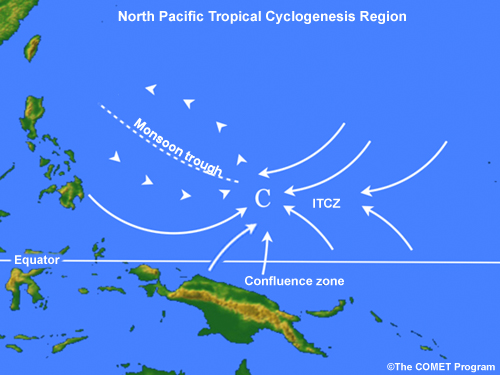
The Western North Pacific monsoon region has the highest frequency of tropical cyclones on Earth, mainly because the tropical western Pacific is the warmest part of the tropical ocean. Tropical cyclogenesis is most common in the monsoon trough (Fig. 3.42, Chapter 8, Section 8.3.2Chapter 8, Section 8.3.2)44 and the location of the monsoon trough has major influence on the distribution of tropical cyclone activity in this region.45 Large-scale cyclonic vorticity in the monsoon trough is derived from the low-level equatorial westerly or southwesterly winds and the subtropical easterly trade winds (Fig. 3.42). Tropical cyclone formation is favored near the eastern end of the monsoon trough and in the confluence zone between the monsoon westerlies and the easterly trade winds (Fig. 3.42). Sometimes a reverse-oriented monsoon trough forms,45 one that extends northeastward from the South China Sea, in the direction of the Mei-yu/Baiu front (Fig. 3.39a). Under those conditions, tropical cyclone activity in the monsoon region is reduced.45 On rare occasions, tropical cyclones formed when the monsoon trough organizes into a gyre.46 While infrequent, once formed gyres can last 2-3 weeks and generate several vortices, the seedlings for tropical cyclones.46 Learn more about tropical cyclones in the monsoon trough in the chapter on tropical cycloneschapter on tropical cyclones.
East Indian Ocean Summer Monsoon systems
The eastern Indian Ocean has its characteristic summer monsoon thunderstorm system, such as the Sumatras. The Sumatras are eastward moving, short-lived squall lines that form over the Straits of Malacca in the low-level convergence between land breezes from Sumatra and Malaya.47 They form at night, during predawn hours, and attain lengths of 200-300 km while moving east to Malaysia and Singapore. Sumatras are critical to the regional rainfall; they produce heavy rain and occur about 3-4 times per month.
The Asian Winter Monsoon
The winter monsoon is stronger over East Asia than over the Indian Subcontinent because of the contrast between the very cold Asian landmass and the warm North Pacific Ocean (the warm Kuroshio Current transports heat from the equator). In addition, the cross-equatorial flow to the Australian-Indonesia monsoon is enhanced by the difference between hot Australia and the relatively cool north Pacific. The north-south contrast is reduced over the Indian subcontinent because the Tibetan Plateau blocks the cold Siberia air mass.
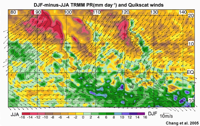
Figure 3.43 shows the difference in TRMM precipitation radar data and QuikSCAT winds between December-January-February (DJF) and June-July-August (JJA) over tropical East Asia. Yellow to red areas get more rain during June-August while green to blue areas get more rain during December-February. During the boreal winter, rainfall occurs well north of the equator (e.g., east of the Philippines and Indochina) but during boreal summer, rainfall is mostly confined to the Northern Hemisphere. The difference can be partly explained by stronger boreal winter monsoon winds that blow directly onshore while few coastal regions face the southwesterly monsoon winds.
The Maritime Continent has its most active convection during the winter monsoon. Cold surges from continental Asia serve as the destabilizing mechanism for widespread, prolonged deep convection. In addition, Borneo vortices, synoptic-scale, low-level cyclonic features49 that, while mostly quasi-stationary can migrate within the southern South China Sea. The region west of Borneo is a common location for mesoscale convective complexes.50 Northeast monsoon winds and the sea breeze interact to produce strong low-level convergence offshore that favors organized mesoscale convection.51
3.5 Monsoons »
3.5.4 Other Monsoons Around the World
3.5 Monsoons »
3.5.4 Other Monsoons Around the World »
3.5.4.1 The Australian-Maritime Continent Monsoon
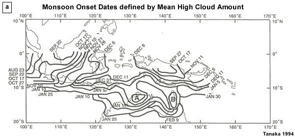
The Australian-Maritime Continent monsoon52 is the seasonal opposite of the Asian Monsoon (note the southern hemispheric warm season in Fig. 3.30 (right panels). Its onset begins over Malaysia in late August and reaches its southernmost extent in early February over northern Australia (Fig. 3.44).
Animation of the Asian-Australian Monsoons,
http://www.cpc.ncep.noaa.gov/products/Global_Monsoons/Asian_Monsoons/Asian_Monsoons.shtml
The monsoon cycle follows the maximum heating as it shifts from its boreal summer location in Asia to the Maritime Continent and northern Australia. The large-scale circulations of the Australia-Indonesia monsoon are not strongly affected by the Earth's rotation because its heat source is near the equator.54 The north-south temperature gradient between the cold Asian land mass and the warm Maritime Continent strengthens cross-equatorial winds.
Much of the precipitation over the Maritime Continent is produced by mesoscale convective systems that are forced by sea/land breezes or large-scale disturbances.50 The proximity of the cold air circulations over continental Asia means that the low-latitude Maritime Continent is affected by cold air outbreaks, which produce instability and deep convection.55 In fact, cold monsoon surges interacting with local circulation were cited as the forcing for a rare near equatorial tropical cyclone, Typhoon Vamei, 2001, at 1.5°N near Singapore.56 Tropical cyclone formation is also favored in the monsoon trough south of the equator during the Australia-Maritime Continent monsoon.57 TC activity in this region is modulated by the interannual ENSO and the intraseasonal MJO. El Niño shifts the monsoon trough to the east along with the rainfall and tropical cyclone activity. The MJO active phase creates a favorable environment for tropical cyclones.58,59 The Australia-Maritime Continent monsoon is explored in more detail in a focus section by Dr. Mick Pope of the Australian Bureau of Meteorologya focus section by Dr. Mick Pope of the Australian Bureau of Meteorology.
3.5 Monsoons »
3.5.4 Other Monsoons Around the World »
3.5.4.2 West African Monsoon
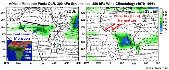
The West African Monsoon (WAM) closely matches for the classical monsoon criteria, with moist, cool southwesterly winds during the summer monsoon and the opposite dry, warm, and dusty northeasterly Harmattan winds during the winter (Fig. 3.45). The Intertropical Front (ITF) or Intertropical discontinuity (ITD) is the boundary between the moist southwesterly monsoon flow and the hot, dry northeasterly wind from the Sahara. Flanking the surface trough are the subtropical high pressure areas of the south Atlantic (St. Helena) and North Africa.
Animation of African monsoon (OLR, 850 hPa winds, 200hPa streamlines),
http://www.cpc.ncep.noaa.gov/products/Global_Monsoons/African_Monsoons/African_Monsoons.shtml
West Africa has a marked south-north gradient in surface conditions with nearly zonal uniformity: from the waters of the Gulf of Guinea, to the equatorial rainforests, to the grasslands and savannah of the Sahel, and, finally to the dry and dusty Sahara (inset map of Fig. 3.45).
The WAM begins along the Guinea coast in early May (Fig. 3.46). The rains end along the Guinea coast by late June into early July (marked by the vertical black lines in Fig 3.46) and the maximum in rainfall shifts to the Sahel. This shift is often referred to as a "jump" and signals the monsoon onset over the Sahel (note trend in time series of rainfall with increasing latitude in Fig. 3.46b). The monsoon begins its southern retreat in late August and the coastal rainy season ends in early November. The WAM monsoon onset date has been linked to the amplification of the SHL, perhaps through orographic interactions with the Atlas and Hoggar Mountains60 of northern Africa.
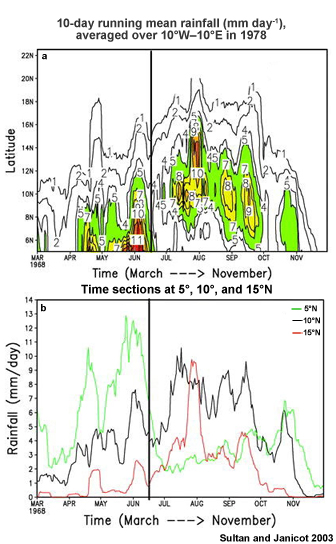
The monthly mean monsoon precipitation cycle and the ITF in the West African Sahel is shown geographically in Fig. 3.47. Notice the strong gradient in precipitation in the Sahel with the northern most areas receiving less than 2 mm day-1 on average even during the peak of the monsoon. The Sahel is known for its extreme variability in precipitation; in a given year, the precipitation band could be north or south of the mean. We will discuss the interannual variability of the WAM in Section 3.5.5Section 3.5.5. Note that the northern boundary of the precipitation is about 100-250 km south of the ITF and the heaviest precipitation is about 400 km south of the ITF. The relationship of the precipitation to the latitude of the ITF, indicates that the ITF could serve as a predictor for the monsoon precipitation advancement and retreat.
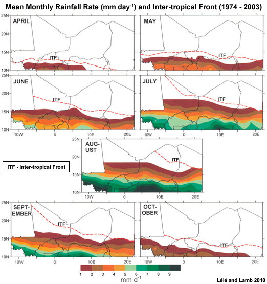
Key features of the WAM are the Sahara Heat Low, the cool SSTs and strong gradients of SST in the Gulf of Guinea, the Sahara Air layer (SAL), the ITCZ, and the mid-tropospheric African Easterly Jet (AEJ)63,64 (Fig. 3.48).
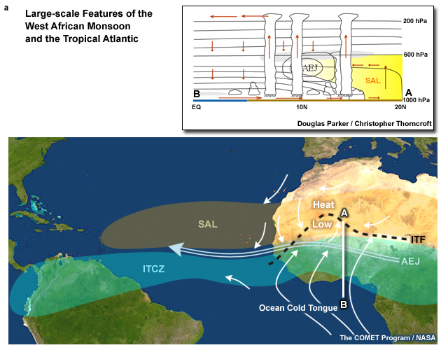
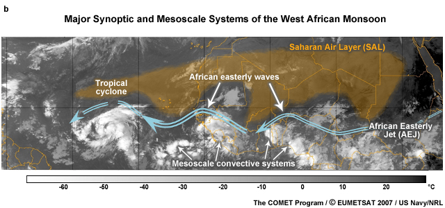
The AEJ is a dynamical response to the unique meridional temperature gradient of tropical north Africa: hot and dry Sahara to the north and cool (ocean/moist soil/vegetation) to the south. The AEJ mean maximum speed is 10 m s-1 near 650 hPa.63 The north-south cross-section (A-B) highlights the contrast in temperature and moisture in the low-mid troposphere (inset of Fig. 3.48a). Strong vertical shear is generated by the AEJ and the low-level monsoon westerlies. The vertical wind shear helps to organize the deep convection represented by the tall clouds in the cross-section. Multiscale interaction is characteristic of the WAM where MCSs, such as squall lines, move with and through synoptic-scale African Easterly Waves (AEW)66,67,68 (Fig. 3.48b). AEWs are ubiquitous phenomena of the African monsoon that occur every 3-5 days and have maximum amplitude at the level of the AEJ. Many Atlantic tropical cyclones form from easterly waves69 and genesis is sometimes the results of easterly wave/MCS interactions (e.g., Fig. 8.24b).70,71 The structure, environments, and lifecycle of West African mesoscale and synoptic systems will be covered in a separate chapter.
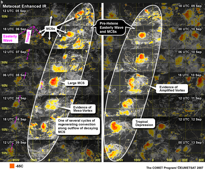
3.5 Monsoons »
3.5.4 Other Monsoons Around the World »
3.5.4.3 Monsoons in the Americas
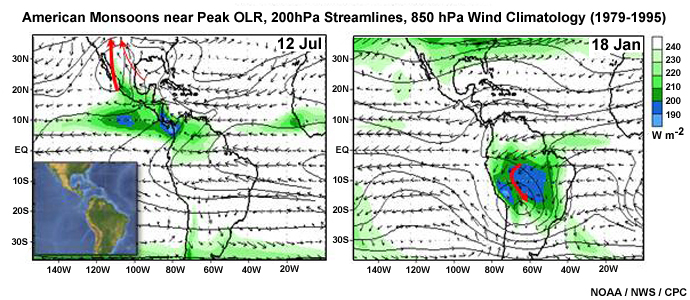
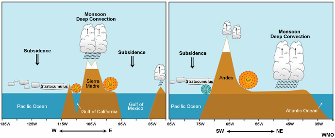
http://www.cpc.ncep.noaa.gov/products/Global_Monsoons/American_Monsoons/American_Monsoons.shtml
The monsoons in the Americas do not match the classical criteria for monsoon as there is no oppositional wind shift during the winter. However there is a reversal in the wind anomalies compared to the annual mean.72
The North American monsoon (NAM) is characterized by heating over the Sonoran Desert and the establishment of a surface heat low into which moist tropical air is drawn from the Gulf of California, Gulf of Mexico (above 850 hPa), and the tropical Pacific (Fig. 3.49, left).73 The South American monsoon (SAM) receives moisture from the tropical Atlantic and Amazon River basin (Fig. 3.49, right).74
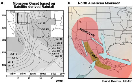
A large portion of the southwestern United States and northern Mexico receives the majority of their annual precipitation during the NAM (about 35-45% for Arizona and 60% for northern Mexico) although most of the NAM rainfall is over the ocean.74 The monsoon rainy season lasts for about 100 days, starting in early June over southern Mexico and reaching its northernmost extent in the high plains of the United States by late July (Fig. 3.50).
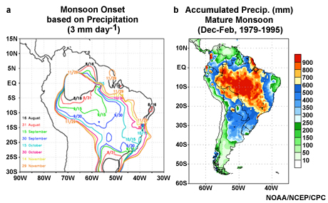
In South America, the monsoon starts in the spring (Fig. 3.51a). Rainfall accumulations reach their maximum over eastern and southeastern during the mature summer monsoon (Fig. 3.51b) and then decrease during the monsoon retreat in autumn.
3.5 Monsoons »
3.5.5 Variability of the Monsoon
Extreme variability in monsoon rainfall leads to devastating floods and droughts,75,76,77,78 major hazards that cause great economic loss and suffering. For example, the African Sahel experienced great loss of life during the 1980s when the monsoon rains were well below normal. Variability of the monsoon is measured by variables such as departure from normal precipitation amounts or dynamical variables such as anomalies of pressure and circulations at various levels. Figure 3.52 shows the major circulation anomalies associated with a strong south Asian summer monsoon and a strong western north Pacific summer monsoon. During strong Indian summer monsoons, the south Pacific subtropical high is stronger, enhancing the cross equatorial flow. The strong western north Pacific monsoon is marked by a wave train pattern that originates in the tropics and emanates towards the North Pacific and into eastern North America, a demonstration of tropical-extratropical interactions and the far-reaching impact of the East Asian monsoon.
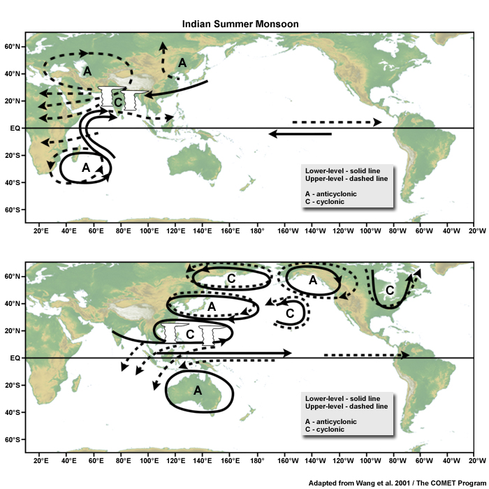
Variations in monsoon intensity over India are measured primarily using precipitation data and, also, using vertical wind shear, which indicates heating differences. Many monsoon indices have been proposed but none are widely accepted, for example,
- Webster and Yang index (WYI) – broad-scale South Asian summer monsoon: vertical shear of zonal wind anomalies between 850mb and 200mb, (40–110E, 0–20N), JJA;
- Monsoon Hadley index (MH) – South Asian summer monsoon: vertical shear of meridional wind anomalies between 850mb and 200mb, (70–110E, 10–30N) JJA;
- All-India monsoon rainfall (AIMR) or Indian Summer Monsoon Rain (ISMR) – Indian summer monsoon rainfall: averaged over Indian continent, JJAS;
- Extended Indian monsoon rainfall (EIMR) – South Asian summer monsoon precipitation including neighboring oceans: (70–110E, 10–30N), JJA.
An increase in the south Asian summer monsoon precipitation occurs with enhancement of the land-sea temperature gradients80 and increased moisture flux to south Asia37,81 (as shown schematically in Fig. 3.53).
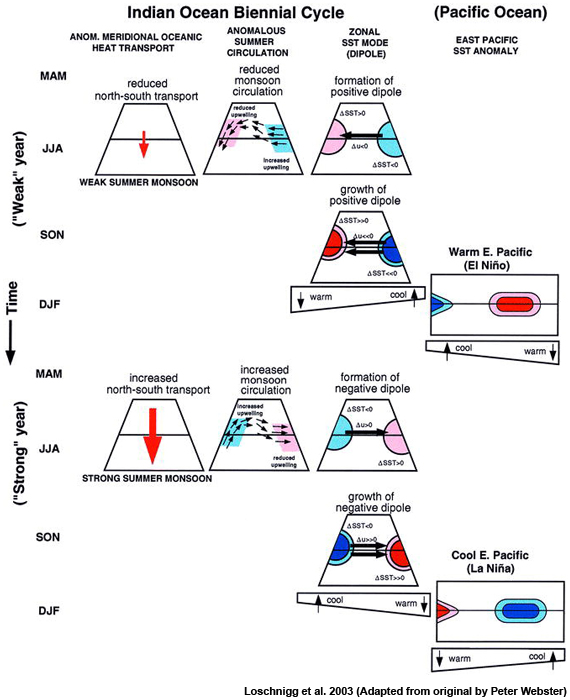
3.5 Monsoons »
3.5.5 Variability of the Monsoon »
3.5.5.1 Tropospheric Biennial Oscillation (TBO) of the Asian Monsoon
The TBO is one of the dominant signals of interannual variability of the Asian-Australian monsoons. It is manifested strongly in summer precipitation and circulations and in the relationships between the Asian monsoon and the El Niño-Southern Oscillation.82 Figure 3.54 illustrates the anomalous changes in the surface winds, convection, SST, Walker Circulation, extratropical circulation, and thermocline depth during the evolution of the TBO. The anomalies shift from south Asia southeastward to southwestern Pacific following the seasons. The tendency is for a relatively strong Indian or Australian monsoon to be followed by a relatively weak one, and vice versa.80,83,84,85,86
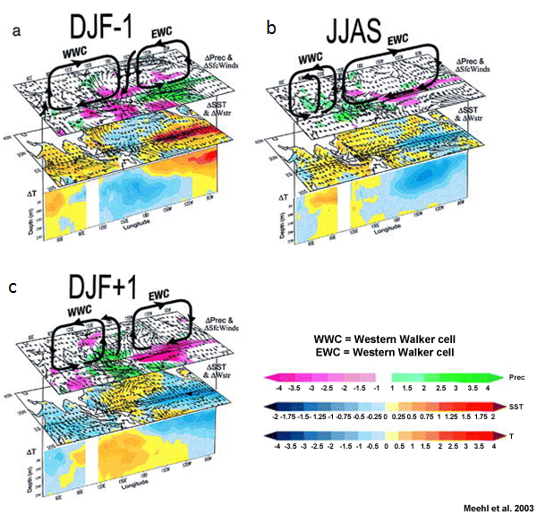
3.5 Monsoons »
3.5.5 Variability of the Monsoon »
3.5.5.2 El Niño-Southern Oscillation (ENSO)
Some interannual variability of the global monsoons is related to ENSO events. ENSO affects the South Asian summer monsoon through the east-west displacement of the Walker circulationWalker circulation and warming over Eurasia. In general, below average rainfall is expected during El Niño, above average during La Niña. However, since the late 1980s, the influence of El Niño events seemed to have weakened.88 In fact, during the extremely strong 1997 El Niño, the Indian summer monsoon rainfall was above normal.89
The East Asian-West North Pacific summer and winter monsoons are strongly influenced by ENSO, even though ENSO is strongest during the boreal winter. SST anomalies in the tropical Pacific that develop during an ENSO cycle induce anomalies in western north Pacific monsoon circulations. During the summer, it leads to east-west elongated anomalies of cyclonic-anticyclonic circulations that form a north-south dipole,90 while during the fall the orientation of the anomalous circulations cells is more NE-SW.
ENSO has a significant impact on the Australian monsoon region. In general, El Niño events are associated with drought (Fig. 3.55), particularly over eastern Australia and negative SST anomalies in the western Pacific and eastern Indian Ocean. ENSO affects rainfall and temperature over Australia, northern Australia tends to be anomalously warm for months following the end of an ENSO cycle. The western parts of Indonesia are weakly correlated with ENSO while the central and eastern regions have good correlation during the rainy season.91 The highest correlation is in the winter hemisphere when rainfall increases over the Maritime Continent during La Niña.
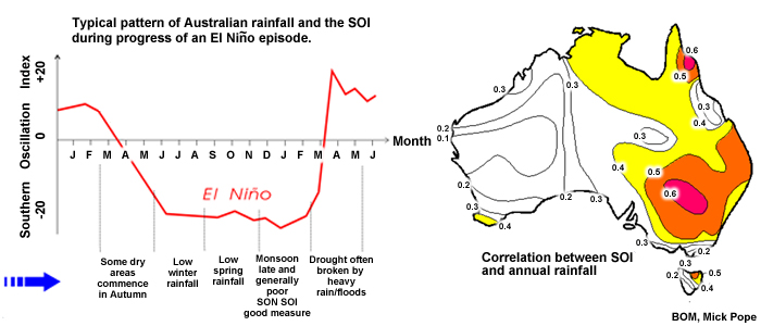
ENSO affects the West African monsoon but with varying correlations since the 1940s.92 The teleconnection between ENSO and the WAM occurs through the modulation of the Walker circulation, which leads to either descent/weak low-level monsoon flow or ascent/strong low-level monsoon flow over tropical West Africa. ENSO has a greater impact when both the Guinea coast and the Sahel precipitation anomalies are the same sign. ENSO correlation is weakly negative during periods when the tropical Atlantic exerts a greater influence; then the Guinea coast and the Sahel have opposite signed rainfall anomalies.93
3.5 Monsoons »
3.5.5 Variability of the Monsoon »
3.5.5.3 Indian Ocean Dipole or Zonal Mode
A major mode of variability in the Asian-Australian monsoons is the Indian Ocean Dipole (IOD) or Indian Ocean Zonal Model (IOZM), an east-west oscillation in SST anomalies that is accompanied by a shift in precipitation anomalies.94,95,96 In general, the positive IOD phase is associated with heavier rainfall over Africa, less over Indonesia; the reverse pattern occurs during the negative phase (Fig. 3.56). Generally, the dipole begins to be evident in early to mid-summer, reaches its peak in late fall to early-winter, then rapidly decays during the boreal spring. The negative phase has similar timing, magnitude, and decay.
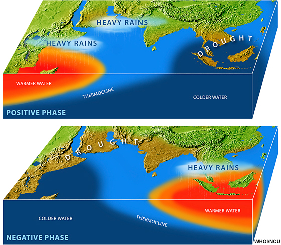
The Equatorial Indian Ocean Oscillation (EQUINOO)89,97 is the atmospheric component of the coupled Indian Ocean Dipole mode. Extreme anomalies of Indian summer monsoon rainfall are correlated with the combined effect of EQUINOO and ENSO. The mechanism(s) for the IOD are still being debated and it is not clear whether it is fully independent of ENSO.78,94
3.5 Monsoons »
3.5.5 Variability of the Monsoon »
3.5.5.4 Interannual Variability of the West African Monsoon
The most important influence on the intensity of the West African monsoon is the thermal contrast between the Gulf of Guinea SSTs and the heated North African continent. The tropical Atlantic exerts a greater direct influence on the West African monsoon than ENSO. The oceanic forcing of the WAM is amplified by land surface-atmospheric feedbacks, e.g., effects of vegetative cover on radiation.98
The dramatic decline in the Sahelian rainfall since the early 1970s (Fig. 3.57) has been extensively studied.93,98,99,100,101 The decline was most extreme in the early 1980s and has been linked to anomalously warm SSTs in tropical ocean basins but especially in the nearby tropical Indian Ocean and tropical Atlantic Ocean. Warm of the eastern Atlantic reduces the land-ocean contrast and onshore monsoon flow into West Africa.
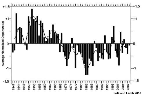
3.5 Monsoons »
3.5.5 Variability of the Monsoon »
3.5.5.5 Intraseasonal Variability
Intraseasonal oscillations are related to active and break periods of the monsoon. During break periods, conditions shift from moist to relatively dry for 1-2 week periods and sometimes for as long as 30 days (Fig. 3.58).
For the South Asian monsoon (Fig. 3.59),
- Active periods occur with strong westerlies: Precipitation is high in the Bay of Bengal and over India but it remains relatively dry over the equator.
- Break period occur within weak westerlies: Precipitation is low in the Bay of Bengal and India, wet over the equator.
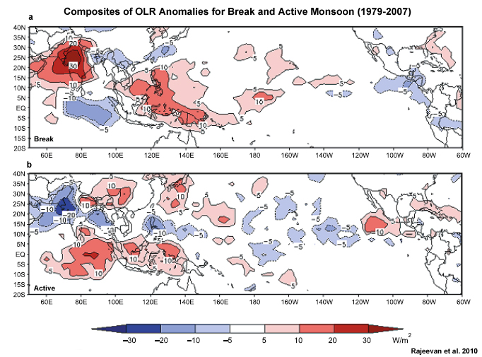
Intraseasonal variation of the south Asian monsoon also features northward propagation of cloud bands from the equatorial Indian Ocean at 2-6 week intervals, which helps to maintain convergence over the continent.103 In the south and east Asian monsoons, the time scale of 10-20 days and 30-60 days are dominant.104,105 The latter is the time scale of the MJO.
Madden-Julian Oscillation (MJO)
The MJOMJO, the 30-60 day oscillation in tropical rainfall and large-scale circulation, is strongest over the Indian Ocean and Pacific Ocean so it should not be surprising that it affects the Asian-Australian monsoons.58,106 The MJO moves eastward and its cycle typically begins with anomalous rainfall over the Western Indian Ocean then propagates across the Pacific where it weakens over the East Pacific but reappears over the Atlantic and continues to the Indian Ocean.107,108 The active phase of the MJO is favorable for monsoon onset over India and Australia, while onset is rare during its suppressed phase.
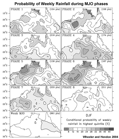
The MJO plays a greater role in the Australia-Indonesian monsoon than elsewhere.110 For example, the probability of extreme weekly rainfall over northern Australia during the wet phases of the MJO is nearly triples that of the dry phases (Fig. 3.60). During the boreal winter,111,112 the MJO often has peak amplitude over the Maritime Continent, which is one of the major tropical heat sources that drive the global circulation (Fig. 1.14a). Consequently MJO-enhanced convection over the Maritime Continent can lead to downstream wave train propagation across the North Pacific, North America, and even to Europe on a one-to-two week time scale.113
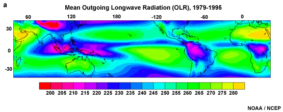
How is the MJO related to the active and break periods of the Australian monsoon? From a study of MJO and Australian monsoon rainfall, it was found that a strong relationship occurred during 1987/88 (R2 = 0.58) but not during 1982/83 (R2 = 0.09). The results indicate that the MJO impact on the monsoon is greater in some years than in others, which may be due to the strength of the MJO in a given year.114
One of the most significant impacts of the MJO during the Australia-Indonesia monsoon is on tropical cyclone activity. More tropical cyclones form during the active phase of the MJO and fewer during the suppressed phase.58,59
The West African monsoon also responds to the MJO. Observational case studies have shown that equatorial waves that are excited by the MJO propagate to West Africa and enhance moist westerly inflow and strong ascent.
Equatorially-trapped waves
Sub-seasonal variability in the Asian-Australian and West African Monsoon is also related to convectively-coupled Kelvin waves and equatorial Rossby waves (Fig. 3.26). Dry/wet spells over West Africa at the 25-60-day time scale have been related to a combination of equatorial Kelvin (e.g., Chapter 4, Fig. 4.15) and Rossby waves forced in the Pacific by the MJO.115, 116
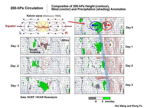
Wet and dry spells in the American monsoons
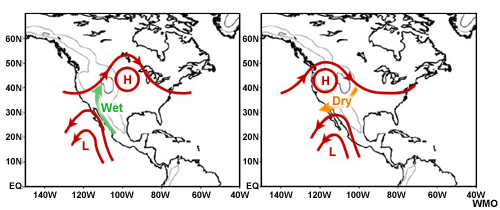
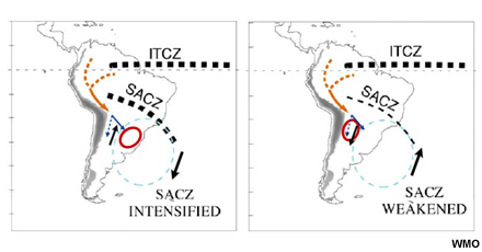
Thunderstorms in the American monsoon systems are triggered by orographic lift and surface heating with inflow enhanced by low-level jets (Fig. 3.49). Like monsoons elsewhere, the North American monsoon thunderstorm activity has "break" and "burst" periods. During the burst periods, a weak trough forms in the upper level westerlies which, in combination with the strong surface heating and moisture convergence, leads to instability and widespread thunderstorm activity. By comparison, the break periods occur when the ridge from the surface Pacific High extends inland, cuts of the southerly flow, and suppresses convection (Fig. 3 .61, upper).
In addition to modulation by the MJO, the South American Monsoon intraseasonal variability is also influenced by the amplitude of moisture flux from the Amazon and the intensity of the South American Convergence Zone117 (Fig. 3.61, lower). Enhanced precipitation over the SACZ is coincident with less rainfall in the subtropical plains. The SACZ is weakened while moisture flux increases from the Amazon and precipitation increases over the inland subtropical plains (Fig. 3.61, lower right).
3.6 Tropical Circulation and Precipitation Distribution
The large-scale circulation features in the tropics affects the distribution of precipitation over tropical ocean basins and nearby continental regions. In general, the subtropical eastern ocean and nearby continent are dry. Moving westward, the subtropical ridge and trade wind inversion weaken, clouds grow taller, and precipitation intensity and amount increase as depicted schematically in Fig. 3.62. The major exception to this rule is the Indian Ocean where monsoon westerlies dominate.
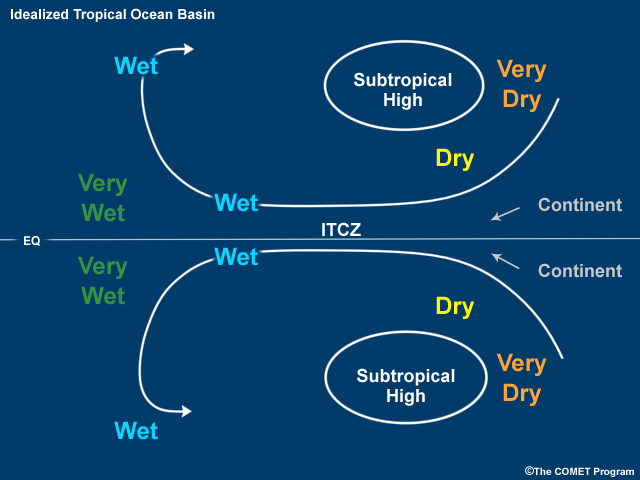
The wettest regions are found over the western tropical ocean basin, the result of pooling of warm surface waters driven by the trade winds. The warmest ocean is the tropical western Pacific, a region known as the Tropical Warm Pool. Heavy precipitation over nearby land results from evaporation from the warm ocean and water vapor being advected downstream. Moderately wet regions are found to the north and east of the very wet areas. Figure 3.63 confirms the conceptual pattern of precipitation and prevailing flow for the tropical Atlantic and Pacific during July and as well as the southeast Indian Ocean during January.
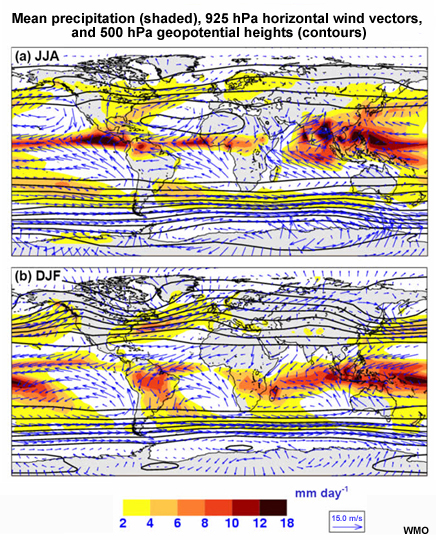
3.7 The Role of the Tropics in the General Circulation
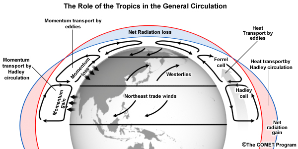
The role of the tropics in the general circulation can be summarized by Fig. 3.64. The tropics serve as a source of surplus heating that drives the global circulation. The transport of heat and momentum by the Hadley Cells is vital to the maintenance of the global heat balance and angular momentum balance. Recent studies have found that the strength of the Hadley and Walker circulations can fluctuate and they actually strengthened during the 1990s.118,119 Scientists related changes in cloud cover and radiation in the regions of subsidence (sinking) and convection (rising) in the circulation cells to changes in the vertical velocity of air. This acceleration of the Hadley and Walker circulations was associated with more thermal, long-wave radiation escaping the tropical atmosphere and a decrease in the reflected sunlight (by about 4 watts per square meter).
Focus Areas
Focus Areas »
Focus 1: Modeling the Global Circulation
Focus Areas »
Focus 1: Modeling the Global Circulation »
3F1.1 Global Models
Numerical models of the global earth-atmosphere system (including land, oceans, ice, and biosphere) are based on the fundamental principles of dynamics and thermodynamics described in Section 3.1Section 3.1 and 3.33.3, such as the equations of motion, continuity principle, ideal gas law, hydrostatic balance, and laws of thermodynamics. Those equations are converted into computer programs and calculated at points on a gridded sphere. Models are initialized using data from surface observations, radiosondes, satellites, ships, and aircraft. The equations are then integrated over a specified time. Figure 3F1.1 is an illustration of a global model output of sea surface temperatures, sea ice concentrations, sea level pressure, and low-level winds. Some processes too complex to represent computationally, or too small to be presented by the grid-spacing of the model, or knowledge of the processes is insufficient to represent the process explicitly. These processes are "parameterized", which means that a numerical estimate is made of their effect rather than modeling the process itself. For example, ocean models include parameterization of small eddies that are too small to be represented by a grid cell (Fig. 3F1.2) because we cannot observe each one or represent them on global model grids. The same can be said of individual clouds. Global models cannot predict individual clouds but strives to provide best approximation of the effects of clouds within the modeled circulation. A schematic of global climate model processes and components is shown in Fig. 1.15.
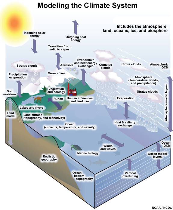
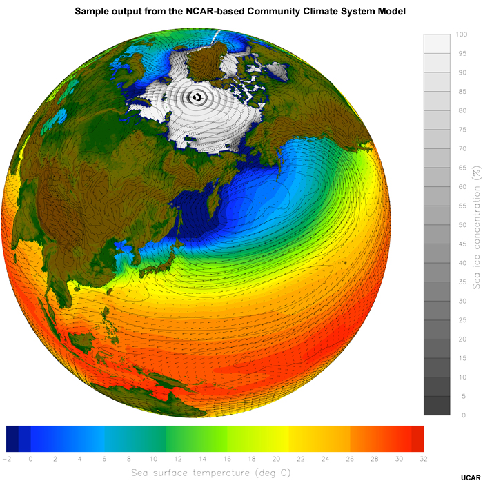
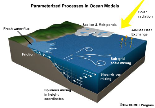
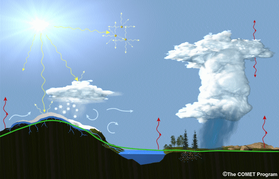
The global models, like other numerical models, have sources of errors including:
- Initial Conditions: Observational data coverage (how much and how often), data error (instrument and representativeness), quality control, errors in how the data is assimilated into the model and objectively analyzed on the model grid, and missing variables
- Numerical Approximations: Errors in the equations used and their numerical approximation, type of grid used (orthogonal, hexagonal, cubed), spatial resolution, time integration steps and procedures
- Boundary Conditions: Surface conditions, vertical boundary conditions, topography
- Physical Approximations or Parameterizations: Clouds (cumulus convection), microphysics (precipitation), radiation, turbulence in the boundary layer
- Intrinsic Predictability Limitations : Fluid motions are chaotic. Numerous scales of motion exist in the atmosphere. Energy from scales smaller than the resolution of the observations is not in the models. Therefore, the real atmosphere and the model atmosphere are different and will diverge over time.
Focus Areas »
Focus 1: Modeling the Global Circulation »
3F1.2 Climate Change and the Thermohaline Circulation
The Gulf Stream transports warm water from tropics to North Atlantic (Fig. 3.20), which keeps Europe warm for its latitude (compare London at same latitude as Hudson Bay and Sweden at the same latitude as Greenland). The Gulf Stream is driven by:
- Wind stress from the North Atlantic Gyre (Fig. 3.20)
- Thermohaline circulation: subduction (sinking of high density water under lower density water) of cold salty water from Arctic, draws up Gulf Stream to replace the water mass lost. (Fig. 3.22b)
Subduction is driven by very cold water produced by long winter nights and by increased water density due to increased salinity of water in contact with the forming Arctic ice. Freezing of ice cap, forces salt out of the ice thereby increasing salinity of water in contact with the developing ice.
Among the predicted scenarios of the consequences of global warming to the Thermohaline Circulation are:
- Ice cap melts creating an excess of floating fresh water in the Arctic Ocean
- Permafrost and glaciers, particularly in Siberia, melt, causing huge flux of warm fresh water into Arctic Ocean via northward draining rivers.
- Low density water inhibits subduction and supply of deep water to the cold conveyor belt
- Gulf Stream slows, and turns east at much lower latitude because it is no longer being driven northward
- Cessation of northward heat transport causes Europe, and northeast North America to become colder.
Since most of the Earth is covered by ocean, the interactions of the ocean on climate are also of interest in a changing climate. Since atmospheric winds produce currents, variations in climatological winds can affect ocean currents, that can affect the transfer of thermal energy and vapor into the atmosphere, that can affect weather and climate, that can affect wind that affects currents and so on. The feedback between climate variability and ocean current variability help to "lock in" certain climate regimes.
Focus Areas »
Focus 1: Modeling the Global Circulation »
3F1.3 Projection of Future Asian Summer Monsoon Changes
The global monsoons are coupled atmosphere-ocean-land system responses to differential heating. Therefore any future changes in the amount of net heating, its spatial and temporal distribution will affect the monsoon systems. However, as noted earlier, the monsoon systems exhibit variability at various scales, creating inherent uncertainty into any projected scenario. Our limited understanding of radiative cloud processes and the feedbacks among the atmosphere, ocean, and land adds further complications.
Among the scenarios projected for future south Asian monsoons (Fig. 3F1.3) is that an increase in global temperatures will lead to:
- An increase in the seasonal mean precipitation of the South Asian summer monsoon because of (1) enhanced land-sea temperature contrast and (2) increased moisture transport into the South Asian monsoon region96,120
- An increase in the interannual variability of the South Asian summer monsoon precipitation that is related to the changes in tropical Pacific SST.96,120
Meanwhile, recent simulations indicate that South Asian summer monsoon circulation may decrease with CO2 increase121 (Fig. 3F1.4). As noted earlier, models differ in complexity and uncertainty so it is not surprising that they can disagree in their projections.
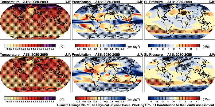
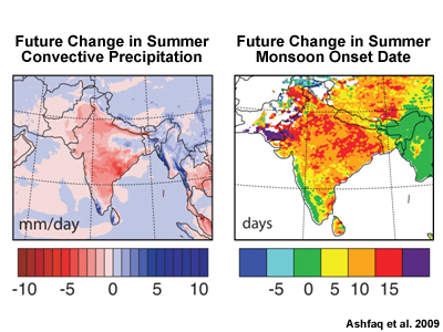
Focus Areas »
Focus 2: Low Level Jets in the Tropics
Low-level jets (LLJs) are regional wind maxima in the lower troposphere that are defined by Stensrud (1996)122 as follows:
- Narrow area of maximum in wind speed below 700 hPa
- Vertical wind profile with speed increasing to the jet core and decreasing above
- Horizontal wind shear exist on side of the jet, e.g., weaker winds at the edge of the jet
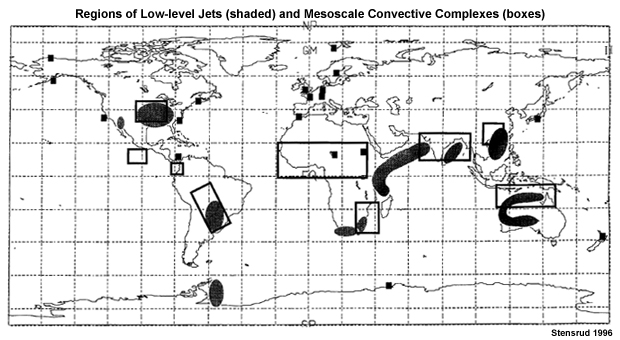
The ribbons of maximum low-level winds are conduits of low-level moisture that feeds organized convection and precipitation (Fig. 3F2.1).122,42,123 Variability in the LLJs can have a large impact on regional precipitation.123,124,125
Among the most well-known of the tropical LLJs is the Somali Jet, a southwesterly jet with maximum speed near 850 hPa that feeds moisture to the South Indian monsoon (Fig. 3.32). The jet results from cross-equatorial flow that is bounded by the East African Mountains to the west (Fig. 3.36). In East Asia, deep convection, and heavy precipitation are persistent where a low-level jet at 850 hPa interacts with the Mei-yu/Baiu front (Figs. 3.39, 3.41a).41,42 The South American LLJ (Fig. 3.49) is a critical part of the precipitation cycle in that continent and variability in its location and intensity have a great impact on warm season precipitation in South America.123
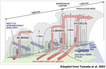
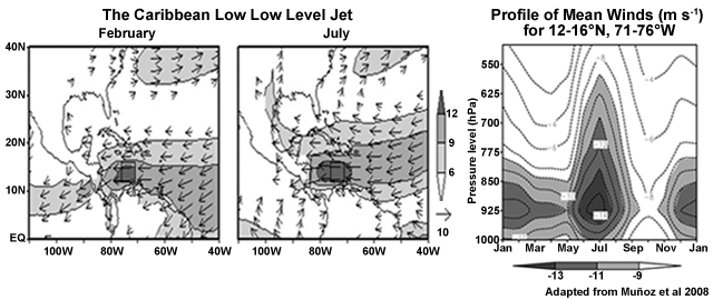
An example of an LLJ in the trade wind regime is the Caribbean Low-Level Jet (CALLJ), an easterly jet with maximum speed at 925 hPa that is prevalent over the Caribbean Sea between 12–14°N and 70–75°W mainly during February and July (Fig. 3F.2.2).124 The CALLJ transports vast amounts of moisture toward Central and North America.124,125
Focus Areas »
Operational Focus
Knowledge of seasonal climatology
- A roadmap to the tropics and subtropics, 3.2.2A roadmap to the tropics and subtropics, 3.2.2
- Tropical precipitation patterns, 3.6Tropical precipitation patterns, 3.6
Streamline analysis
- Identify convergence and divergence, 3.1.5Identify convergence and divergence, 3.1.5
- Identify curvature and shear vorticity, Fig. 3.8
Regional monsoon onset and evolution
- Conceptual Model of Monsoon Evolution, 3.5.2Conceptual model of monsoon evolution, 3.5.2
- Asian Summer Monsoon Onset Dates, Fig. 3.34
- Australia-Maritime Continent Onset Dates, Fig. 3.44
- North America Monsoon Onset, Fig. 3.50a
- South American Monsoon Onset, Fig. 3.5 1
- West African Monsoon Onset, Fig. 3.46, 3.47
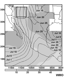
Monsoon weather systems
- Mei-yu/Baiu Front and Weather Systems, 3.5.3 Mei-yu/Baiu front and weather systems, 3.5.3
- Winter Monsoon Convection in East Asia, 3.5.3Winter monsoon convection in East Asia, 3.5.3
- Maritime Continent Monsoon Convection, 3.5.4.1, 3.5.3Maritime Continent monsoon convection, 3.5.4.1, 3.5.3
- Major Weather Systems of West African Monsoon, 3.5.4.2 Major weather systems of West African monsoon, 3.5.4.2
Monsoon regions and tropical cyclone genesis
- Monsoon Trough and Tropical Cyclone Genesis, 3.5.3Monsoon trough and tropical cyclone genesis, 3.5.3
- Tropical Cyclones in the Australia-Maritime Continent Monsoon, 3.5.4.1 Tropical cyclones in the Australia-Maritime Continent monsoon, 3.5.4.1
- West Africa and Atlantic, 3.5.4.2 West Africa and Atlantic, 3.5.4.2
Forecasting breaks during the monsoon
- Wind Shifts during Active and Break Monsoon Periods in South Asia Wind shifts during active and break monsoon periods in South Asia
- MJO Impacts on Monsoon, 3.5.5.5 MJO impacts on monsoon, 3.5.5.5
- Wet and Dry spells in the American Monsoons, 3.5.5.5 Wet and Dry spells in the American monsoon system, 3.5.5.5
How monsoons vary from year to year
Summary
The tropics serve as a source of surplus heating that drives the global circulation. The transport of heat and momentum by the Hadley cells is vital to the maintenance of the global heat balance and angular momentum balance. Atmospheric and oceanic circulations are governed by basic principles, such as the equations of motion, the conservation of mass, energy, and angular momentum. The historical evolution of the general circulation models from Halley in the 17th century through until present day showed that with a few observations much can be deduced about the mean balanced flow. Theoretical studies showed that the Hadley cell extent is constrained by the static stability in the subtropics and the subtropical jet, which is itself controlled by angular momentum conservation. From the theoretical concepts, we can describe the seasonal progression of the Hadley circulations including the ITCZ, differences between northern and Southern Hemisphere. The tropics are also described in terms of the contrast between tropical and the midlatitude wind systems.
In this chapter, we examined the mechanisms for the monsoon systems including the migration of surplus heating and associated precipitation, the initiation of a planetary-scale sea breeze system, moist convective processes, and cross-equatorial heat transport. We learned that the monsoon is highly variability during the season with active and break periods associated with the MJO, equatorial waves, and oscillations of the subtropical highs, and convergence zones. At the interannual scales and beyond, the variability is highly influenced by the ocean temperature gradients and interactions with ENSO, especially for the East Asian, Australian, and Maritime Continent. Monsoon systems are noted for bringing heavy rainfall that is beneficial for agriculture and hazardous when it leads to flooding. Numerical models of the global circulation are based on the basic dynamic and thermodynamic principles of the atmosphere and ocean. However, the models have sources of errors such as those associated with the parameterization of processes that are too complex to be represented computationally, are sub-grid scale, or are too poorly measured or understood. The uncertainty in the global models varies regionally with higher levels of uncertainty over the tropics.
Questions for Review
- Explain why geostrophic balance is not a good approximation for motion at the equator.
- Explain why the hydrostatic approximation is not applicable for tropical convective systems.
- Describe how the continuity principle relates divergence/convergence to pressure, vertical motion, and expected weather.
- Compare the typical balance of forces for horizontal motion in the tropics to the force balance in the midlatitudes.
- How is the Hadley cell maintained and what are the controls on its latitudinal extent?
- Compare and contrast the northern and southern hemispheric pressure and wind systems in the tropics and subtropics.
- List at least three differences between atmospheric motion in the tropics and the midlatitudes.
- Describe the ITCZ, its role of the general circulation, and the mechanisms that influence its location
- What is the role of the tropics in the global stratospheric circulation?
- Define the tropical tropopause layer and describe its role in global-scale chemical transport.
- Describe the theoretical basis for the Walker Circulation as a response to differential heating at the equator.
- How can the Hadley circulation be considered as a response to differential heating in the tropics?
- Describe how Ekman transport influences weather and climate in the tropical Pacific region.
- Describe the major factors that in combination create the global monsoon systems.
- List the criteria for the classical monsoon and describe the monsoon systems that match or do not match those criteria.
- Describe the evolution of the Asian monsoon from onset to demise in terms of precipitation and mean synoptic-scale features.
- What is the influence of the MJO on the variability of global monsoon systems?
- Describe the modes of interannual variability in the Asian monsoon including the role of the Indian and Pacific Ocean SSTs.
- Describe the major factors that lead to intraseasonal variability and break periods in the Asian-Australian monsoons.
- What are some conditions in monsoon regions, such as West Africa and East Asia, that make those regions conducive to tropical cyclone genesis?
- What are some sources of intraseasonal variability in the American monsoon systems?
- Describe the typical pattern of precipitation over the tropical oceans including the role of surface winds and ocean currents.
- Describe the role of the tropics in the general circulation including the transport of heat and momentum.
- List the major components of a general circulation model.
- Describe major sources of errors in general circulation models.
QUIZ
You may also take a quiz and email your results to your instructor.
Brief Biographies
James Sadler (1920-2005)
James Sadler was a founding father of tropical meteorology and the discoverer of the Tropical Upper Tropospheric Trough, work for which he was honored by the American Meteorological Society in 1978. He turned his experience working for the Air Force in meteorology into a life-long devotion to tropical meteorology. He was born in 1920 in Silver Point, Tenn., and graduated from Tennessee Polytechnic Institute in 1941 with a civil engineering degree. He earned a meteorology certificate from M.I.T. in 1942 and a master’s degree in meteorology from the University of California in 1947. He applied his World War II meteorology training to satellite observations, working on the first TIROS weather satellite as chief of the Air Force’s satellite branch. He spent over two decades as a meteorologist with the Air Force before joining the University of Hawaii as an associate meteorologist. He retired there 22 years later as a professor of tropical meteorology, having devoted himself to understanding tropical weather and climate. While there, he was the author of many books, including The Upper Tropospheric Circulation over the Global Tropics. By studying pressure maps, Sadler discovered a trough over the eastern and central North Pacific and learned this upper-tropospheric circulation was a force in the birth and development of tropical cyclones. His understanding and analysis of tropical meteorology were almost without equal, his students remember. One told the Honolulu Star-Bulletin, "He could also extract more information from a satellite image than anyone I've ever met—even in cloud-free regions!"
Colin Ramage
Colin Ramage was the first director of the Department of Meteorology at the University of Hawaii Manoa and the author of the classic textbook, Monsoon Meteorology. He was recruited to Hawaii from his position as deputy director of the Royal Observatory in Hong Kong after a 1956 Air Force grant for research on Pacific typhoons led to the creation of a meteorology training program and library at the university. He served as director until he retired in 1988. During his tenure, he oversaw the development of the program from six-week training courses for government meteorologists to a world-class Ph.D. granting institution. He also participated in an oceanographic expedition to the Indian Ocean where he headed the meteorological research program. This voyage was an impetus for his classic textbook. In 1981 he traveled to the University of Colorado to be a visiting fellow in the Cooperative Institute for Research in Environmental Sciences (CIRES) program where he helped do early important work on climate change and ocean climate. From 1985 to 1990 Ramage was active in studies of the El Niño Southern Oscillation and served as a member of the Council for Equatorial Pacific Ocean Climate Studies, later the Tropical Ocean Global Atmosphere project.
Sulochana Gadgil
Sulochana Gadgil, a professor at the Indian Institute of Science, is an expert in the workings of the Indian Monsoon, ocean dynamics, and how the two interact. Born in Pune, India, in 1944, Dr. Gadgil’s father, a physician, fostered her interest in science and mathematics. She received a bachelor’s degree in chemistry in 1963 from Poona University and a master’s degree in applied math in 1965. She traveled to Harvard University for her Ph.D., which she earned in 1970 for her research on Gulf Stream fluid dynamics. The next year she worked as a research fellow at M.I.T. In 1971 she moved back to Pune to work as a pool officer for the Council of Scientific and Industrial Research at the Indian Institute of Tropical Meteorology. In 1973 she accepted a faculty position at the Indian Institute of Science in Bangalore. She continues to hold that post today. Her work has examined the monsoon’s rainfall patterns, associated regional climate changes, and the effects of monsoonal precipitation on farming. In 1980 she won the India Career Award and, in 1982, the B.N. Desai Award of the India meteorological Society. She is also a fellow of the Indian Academy of Science.
Peter Webster
Peter Webster is a professor at Georgia Tech who has made great contributions to research at the intersection of ocean and atmosphere, particularly in the tropics. His contributions have been recognized with various awards including the top two awards of the American Meteorological Society (AMS): the Jules G. Charney award in 1990 and the Carl Gustav Rossby Research Medal in 2004. He is a Fellow of the AMS, the American Geophysical Union (AGU), the American Association for the Advancement of Science (AAAS), and the Royal Meteorological Society. Webster earned his Ph.D. at M.I.T. in 1972. From 1973-1977 he was an assistant professor in the Department of Atmospheric Sciences at the University of Washington at Seattle. He became a full professor while in the Department of Meteorology at Pennsylvania State University (1983-1992) followed by directorship of the Program in Atmospheric and Oceanic Sciences at the University of Colorado (1992 to 2000) and recently to his current position at Georgia Tech. He was the lead scientist of the successful international Tropical Ocean Global Atmosphere- Coupled Ocean Atmosphere Response Experiment (TOGA COARE) field research program. In recent years, he has focused on the Asian monsoon as well as tropical cyclones. Webster was among the first scientists to deduce that climate change might be contributing to the strengthening of the strongest hurricanes as a result of warmer surface waters.
John McBride
John McBride is a Senior Principal Research Scientist with the Bureau of Meteorology at its Centre for Atmospheric Weather and Climate Research in Melbourne, Australia. He is an expert on monsoons—particularly the Australian and South East Asian monsoons—tropical cyclones, tropical heating profiles, and tropical convection. He earned an M.Sc. in Physics from the University of Melbourne and a Ph.D. in Atmospheric Science from Colorado State University. He was Head of Climate Forecasting Research at the Bureau of Meteorology from 2005-2007 and was also Head of Weather and Environmental Prediction Research for the Bureau and CSIRO Joint Research Centre (CAWCR) from 2007-2009. In the course of his career, he has written about 70 papers in international refereed scientific journals. He wrote a seminal paper showing the relationship between Australian rainfall and the El Niño Southern Oscillation in the early 1980s with co-author Neville Nicholls. He has also co-authored pioneering papers on the use of genesis indices to forecast tropical cyclone development and on entity-based methods for rainfall verification. Currently, he co-chairs the World Weather Research Programme Expert Team on Climate Change Impacts on Tropical Cyclones and is a lead scientist for the Bureau of Meteorology Indigenous Weather Knowledge project.