Table of Contents
- 4.0 Overview
- 4.1 Sources of Intraseasonal Variability
- 4.2 Sources of Interannual Variability
- 4.2.1 The El Niño-Southern Oscillation (ENSO)
- 4.2.1.1 Description of the Walker Circulation
- 4.2.1.2 ENSO Evolution
- 4.2.1.3 ENSO Theory
- Box 4-5 ENSO Behavior and Coupled Ocean-Atmosphere Models
- 4.2.1.4 Monitoring ENSO evolution
- 4.2.1.5 Indices used to Monitor ENSO Evolution
- 4.2.1.6 Comparing El Niño and La Niña atmospheric and oceanic anomalies
- 4.2.1.7 Climate Impacts Related to ENSO
- 4.2.1.8 Forecasting ENSO
- 4.2.2 The Quasi Biennial Oscillation (QBO)
- 4.2.1 The El Niño-Southern Oscillation (ENSO)
- 4.3 Sources of Decadal Variability
- Focus Areas
- Summary
- Appendix A: Solving for the Equatorial Wave Form Solutions
- A1 Derivation of the Shallow Water Equations
- A1.1 Assumptions Implicit in the Shallow Water Equations (SWE) Derivation
- A1.2 Derivation of the Shallow Water Equations in a Rotating Reference frame
- A1.3 The Shallow Water Equations on an Equatorial β -Plane
- A1.4 Linearizing the Shallow Water Equations on an Equatorial β -Plane
- A1.5 Potential Vorticity Equation for Equatorial β-Plane Shallow Water Equations
- A1 Derivation of the Shallow Water Equations
- Appendix B: Derivation of Generalized Dispersion Relation for Waves in the SWE
- Appendix C: Equatorial Wave Motion and Structure
- Questions for Review
- Brief Biographies
- References
4.0 Overview
This chapter presents an overview of major cyclical patterns that dominate tropical intraseasonal and interannual variability, including the impact on higher latitudes. The potential role of multidecadal oscillations in modulating these shorter cycles will be discussed. Characteristic atmospheric and oceanic patterns for the oscillations are presented and methods for tracking their evolution are described. Classical solutions for tropical waves are presented and the effects of moisture on these waves are discussed.
Print Version
The print version provides a single printable page with all required content.
Multimedia Version
The multimedia version provides structured page navigation.
Focus Areas
Quiz and Survey
Take a quiz and email your results to your instructor.
After completing this chapter, please submit a User Survey.
4.0 Overview »
Learning objectives
At the end of this chapter, you should be able to:
- Describe the basic structure and time scale of the MJO
- Understand the mechanisms that form the MJO
- Understand the role of the MJO in atmospheric and oceanic variability
- Describe the general characteristics of equatorial waves (Kelvin Waves, Rossby Waves, Mixed Rossby-Gravity Waves) including length scale, duration and speed
- Describe equatorial wave formation mechanisms graphically or mathematically
- Describe the Walker Circulation
- Define the Southern Oscillation Index
- Describe ENSO in terms of onset, maximum amplitude, and duration
- Describe the previous and current theories of ENSO (from Bjerknes to recent theories such as the delayed oscillator theory)
- Compare and contrast the warm phase (El-Niño) and cold phase (La Niña) patterns in terms of atmospheric and oceanic anomalies across the equatorial Pacific
- Describe at least five climate impacts of El Niño (e.g., drought in Australia, heavy rains in Peru, more winter cyclones across the southern US and the Caribbean, less hurricanes in the Atlantic)
- Describe at least five climate impacts of La Niña (e.g., increased rainfall in West Pacific, drier winter in the southeastern US, wetter summers in the Caribbean and Central America)
- Define the Quasi Biennial Oscillation
- Describe its impact on tropical climate (e.g., influencing seasonal tropical cyclone formation)
- Provide a brief description of the Pacific Decadal Oscillation, the Atlantic Multidecadal Oscillation, and the North Atlantic Oscillation
- Describe one mechanism by which the tropics can force decadal extratropical variability
- Describe at least one impact of decadal fluctuations on interannual and intraseasonal variability
4.1 Sources of Intraseasonal Variability
How can you tell the difference between the tropics and the midlatitudes? By the scales of motion in the atmosphere and the energy associated with transient weather phenomena such as cyclones. For example, the midlatitude atmosphere is often unstable because of air masses with contrasting temperature and density. In the areas where air masses interact, energy is concentrated into extratropical cyclones. In comparison, the tropical atmosphere is relatively homogeneous, so that, except for tropical cyclones, local and mesoscale effects are more dominant than synoptic influences. Many scales of motion interact to transport energy, moisture, and momentum within the tropics and between the tropics and the midlatitudes.
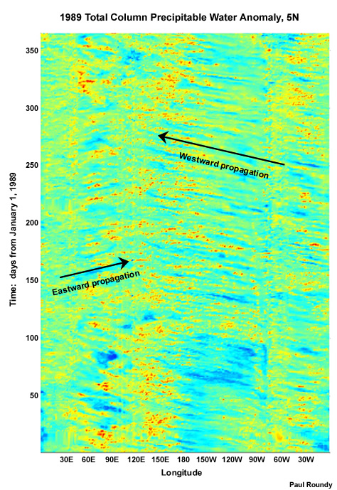
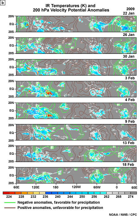
Here, we explore sources of variability in the tropics on timescales ranging from intraseasonal, to a few years, and decades. First, we examine major sources of tropical variability on timescales less than a season, the Madden Julian Oscillation (MJO) and tropical waves (e.g., Fig. 4.1), then increasing in timescale to the El Niño-Southern Oscillation (ENSO) and the Quasi-Biennial Oscillation (QBO) of the stratospheric winds, and finally, decadal variability, such as the Atlantic Multidecadal Oscillation.
Here, we explore sources of variability in the tropics on timescales ranging from intraseasonal, to a few years, and decades. First, we examine major sources of tropical variability on timescales less than a season, the Madden Julian Oscillation (MJO) and tropical waves (e.g., Fig. 4.1), then increasing in timescale to the El Niño-Southern Oscillation (ENSO) and the Quasi-Biennial Oscillation (QBO) of the stratospheric winds, and finally, decadal variability, such as the Atlantic Multidecadal Oscillation.
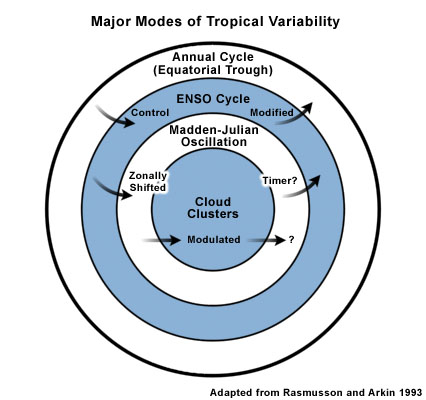
The major sources of tropical variability and their interactions are depicted as a schematic in Fig. 4.2. In the regime between cloud clusters and the MJO we include tropical waves.
For the most part, atmospheric transport of heat and moisture across latitudes is accomplished through meridional transport in the Hadley cells; warm air rises in thunderstorm systems in the tropics, cools, and sinks in the subtropics. Regions of heating and strong convection are observed over the tropical continents and warm ocean basins. Zonal circulations also arise from this convection. In this chapter, we seek to understand the weather and climate phenomena that are generated in response to these heating maxima in order to gain a complete picture of the tropical atmosphere.
4.1 Sources of Intraseasonal Variability »
4.1.1 The Madden-Julian Oscillation (MJO)
The Madden-Julian Oscillation (MJO)a was first identified in 1971 and documented shortly thereafter.2,3 The MJO has been demonstrated to influence tropical weather from small-scale tropical convection through to planetary-scale circulations.4 In this section we will describe the basic structure and time scale of the MJO, examine the mechanisms that form the MJO and seek to understand the role of the MJO in atmospheric and oceanic variability.
a The MJO was originally referred to as the 40-50 day oscillation. However, this period is not precise, so it is also referred to as the 30-60 day oscillation or the intraseasonal oscillation.
4.1 Sources of Intraseasonal Variability »
4.1.1 The Madden-Julian Oscillation (MJO) »
4.1.1.1 Basic Spatial and Temporal Structure of the MJO
In the early 1970s, analyses of observations from around the tropics revealed that surface pressure and atmospheric winds tend to go through a coherent cycle at many tropical locations over periods ranging from 30 to 60 days.2,3,5,6 Subsequent research has tied these variations to alternation of broad active and inactive tropical rainfall in both the Northern and Southern hemispheres: a broad area of active cloud and rainfall propagates eastwards around the equator at intervals of between about 30 to 60 days. Rainfall in the near-equatorial regions of the Indian and Pacific Oceans also show a strong association with the disturbance (Fig. 4.3).
The MJO is a coupled ocean-atmosphere system. The atmospheric component is characterized as an oscillation propagating eastwards from the Maritime Continent around the equator7 at about 5 m s-1; this gives the atmospheric MJO a period of roughly 30-60 days. The spatial scale of the atmospheric MJO can be described in terms of a local wavelength of roughly 12,000-20,000 km. The MJO is generally best developed in the region from the southern Indian Ocean eastward across Australia to the western Pacific Ocean in austral summer. The atmospheric signature is evident in the surface pressure, the lower and upper tropospheric wind strength (or divergence) and in fields representative of deep convection (such as relative humidity, OLR or precipitable water). The wave is not evident in the mid-tropospheric winds.2,3,4
The oceanic component of the MJO has an oscillation with a somewhat longer period of 60-75 days. The oceanic signature of the MJO is evident in the sea surface temperature (SST), mixed layer depth, surface latent heat flux and surface wind stress fields.
The MJO is evident in at least four atmospheric fields and another four fields relating to the ocean. Try to list all eight fields for yourself. (Type your response in the box below.)
To see some of these fields used to monitor the MJO, see the websites maintained by the:
US Climate Prediction Center (CPC), http://www.cpc.ncep.noaa.gov/products/precip/CWlink/MJO/mjo.shtml
Australian Bureau of Meteorology MJO monitoring, http://www.bom.gov.au/climate/mjo/
Can you reconcile the relationships between the atmospheric and oceanic MJO signatures? For example, would you expect the passage of convection to have any impacts on the ocean? (Type your response in the box below.)
Feedback:
In the near-surface, the atmospheric component of the MJO is characterized by enhanced or suppressed westerlies and deep convection. These are the factors that are most likely to influence, or be influenced by, the oceans. Recall that the oceanic signature of the MJO is evident in the SST, mixed later depth, surface latent heat flux and surface wind stress fields. The wind stress will obviously be modulated by the changing westerly surface wind anomalies. The surface latent heat flux and the SST will be modulated by both the surface wind anomalies and the convection. Convection in the active phase of the MJO will cool the SST by reducing the incoming solar radiation and by depositing cool rain water into the ocean surface. This cooling, as well as variations in surface wind stress, will modify evaporation from the ocean—all of these processes contribute to the net influence of the MJO on the surface latent heat flux. The SST and the mixed layer depth will also be modulated by the passage of internal oceanicwaves forced by wind variations on this time scale.
See Section 4.1.1.2 for more on this topic.
See Section 4.1.1.2 for more on this topic.
A composite of 91 MJO events observed at Darwin in the austral summers of 1957-19878 reveals an oscillation with magnitudes of order 5 m s-1 in zonal wind, 1 m s-1 in meridional wind, 0.5 K in temperature, 5 mm day-1 in rainfall and 10% in relative humidity. The temperature and humidity anomalies can be visualized in terms of a vertical profile of equivalent potential temperature, θe (Fig. 4.4). These three profiles are indistinguishable in the planetary boundary layer; indeed, the differences between the active and break convection periods shown only become evident above 700 hPa.9
The atmospheric oscillation associated with the MJO has a baroclinic structure with upper tropospheric warming and cooling in the near surface layer during the westerly phase, with westerly anomalies extending up to 300 hPa. This is consistent with mid-tropospheric latent heating (typical of deep convection) and lower tropospheric cooling due to evaporation of rain; this rainfall event leads the arrival of the westerly anomalies by about 4 days.8
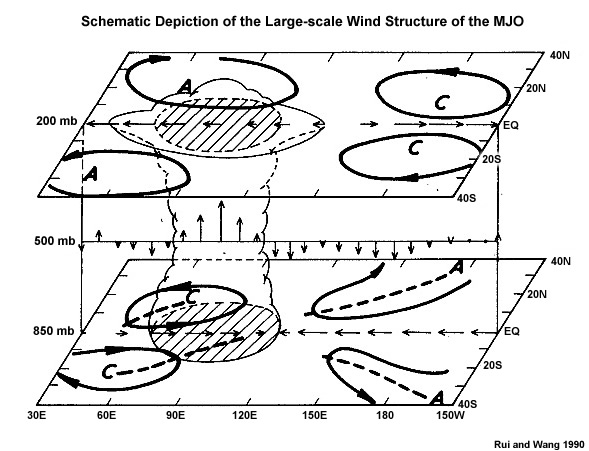
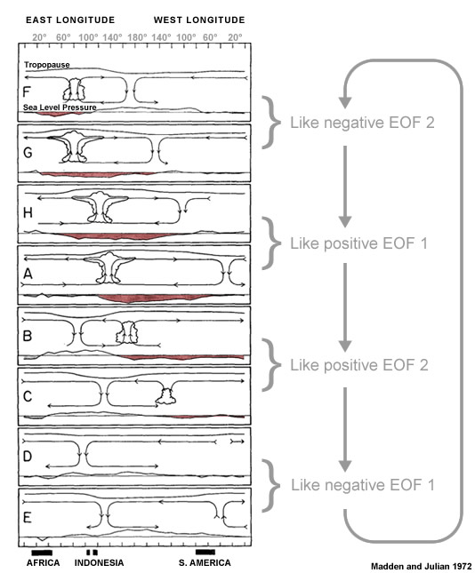
The rainfall leading the maximum in the westerly surface wind anomalies corresponds to enhanced convergence under the convection. This baroclinic structure of the MJO is depicted schematically in Fig. 4.3: panels F through A follow the passage of the westerly, "wet" phase and panels A through E track the easterly, "dry" phase of the MJO through the west Pacific warm pool region. The westerly phase of the MJO is characterized by eastward propagation of convection, anomalously low surface pressure, westerly lower-tropospheric zonal wind anomalies and easterly upper-tropospheric zonal wind anomalies. The easterly phase of the MJO is characterized by suppressed convection, anomalously high surface pressure, easterly lower-tropospheric zonal wind anomalies and westerly upper-tropospheric zonal wind anomalies. Clearly then, this baroclinic structure corresponds to modulations of the Walker cells around the tropics.
If we could travel around the equator with the MJO, we would see that surface air flows away from the suppressed convection in both zonal directions towards enhanced convection regions (i.e. low-level moisture convergence in the region of enhanced convection). Anomalous upper tropospheric divergence is also observed in the enhanced convection region, resulting in anomalous easterlies (westerlies) to the west (east) of the convection. The strong westerlies to the east increase the shear and subsidence in the region of suppressed convection upstream.
The net effect of these wind anomalies is that upper tropospheric anticyclonic gyres are observed to the west of the enhanced convection once it becomes strong in the Indian and western Pacific Oceans. When the convection is suppressed in the Indian Ocean to the central Pacific Ocean, anomalous upper tropospheric cyclonic gyres are detected to the west. Much weaker anomalous (anti-)cyclone patterns are observed at surface. The net effect of these anomalies is to produce a pattern of expanded and contracted latitudinal range of the MJO around the equator (Fig. 4.5).
Predictability in the tropics is inherently poor since balance constraints (such as geostrophic balance) do not dominate atmospheric motionsb in this region. Thus, daily forecasts have the potential for great improvement if a coherent signal or balance condition governing tropical motions can be identified. The MJO is just such a tropical modulator.
The Madden-Julian Oscillation Life Cycle presented by Dr. Roland Madden,
http://www.meted.ucar.edu/climate/mjo/
Australian Bureau of Meteorology (BOM) MJO information page,
http://www.bom.gov.au/bmrc/ocean/JAFOOS/POAMA/scientific/mjo/mjo.htm
b This lack of balance arises since the Coriolis parameter is zero at the equator and small in the deep tropics. Synoptic and mesoscale systems such as tropical cyclones and mesoscale convective complexes are exceptions.
4.1 Sources of Intraseasonal Variability »
4.1.1 The Madden-Julian Oscillation (MJO) »
4.1.1.2 Mechanisms for Formation and Modulation of the MJO
The MJO exhibits large year-to-year variations in intensity.11,12 The impact of the MJO on the tropical circulation means that understanding its interannual variability is important to understanding the variability of the global tropics.
So, what causes the MJO? Initially, scientists believed that the latent heat release from tropical convection was responsible. Matsuno and, later, Gill documented the structures of tropical waves13 and showed how they could be forced by convection.14 One of these waves, the equatorial Kelvin wave, propagates eastwards like the MJO (see Section 4.1.2-4.1.5 for more on equatorial waves). However, the equatorially trapped Kelvin wave travels much more quickly than the MJO (convectively-coupled Kelvin waves have phase speed of ~12-22 m s-1), circling the equator in about a week, rather than the 30-60 day period typically associated with the MJO. This inconsistency in the Kelvin wave and MJO propagation speeds led investigators to explore other explanations for the MJO.
So, what causes the MJO? Initially, scientists believed that the latent heat release from tropical convection was responsible. Matsuno and, later, Gill documented the structures of tropical waves13 and showed how they could be forced by convection.14 One of these waves, the equatorial Kelvin wave, propagates eastwards like the MJO (see Section 4.1.2-4.1.5 for more on equatorial waves). However, the equatorially trapped Kelvin wave travels much more quickly than the MJO (convectively-coupled Kelvin waves have phase speed of ~12-22 m s-1), circling the equator in about a week, rather than the 30-60 day period typically associated with the MJO. This inconsistency in the Kelvin wave and MJO propagation speeds led investigators to explore other explanations for the MJO.
Even after over 35 years of study, doubt remains as to the source of the drivers for the MJO. The two big picture options are that it is (1) internally or (2) externally forced. If it is internally forced, the MJO is responsible for creating its own energy source (running an MJO-driven feedback process). An externally forced MJO would rely on other phenomena for its continued survival. So which is it?
We will briefly review how internal and external forcings might lead to a 30-60 day oscillation in tropical convection symptomatic of the MJO. Interested readers should consult Zhang (2005)6 for a much more complete review.
External forcing theories
Theories proposed for external forcing of the MJO include (1) Intraseasonal fluctuations of the Asian summer monsoon; (2) "stochastic forcing" from convection in the region of the MJO peak; and (3) forcing from the midlatitudes.
The theory for intraseasonal fluctuations in the Asian monsoon forcing the MJO relies on an interaction among surface evaporation, convection, and radiation leading to a stationary oscillation in monsoon precipitation with a period close to 50 days.15 This oscillation provides large-scale convective heating on this period, which could force the MJO, following the idea that this heating would force equatorial waves.13,16 However, neither statistical17 nor modeling18 studies have been able to support this theory. We will explore equatorial wave theory, observations, and forecast in Section 4.1.2-4.1.5.
The theory for intraseasonal fluctuations in the Asian monsoon forcing the MJO relies on an interaction among surface evaporation, convection, and radiation leading to a stationary oscillation in monsoon precipitation with a period close to 50 days.15 This oscillation provides large-scale convective heating on this period, which could force the MJO, following the idea that this heating would force equatorial waves.13,16 However, neither statistical17 nor modeling18 studies have been able to support this theory. We will explore equatorial wave theory, observations, and forecast in Section 4.1.2-4.1.5.
Short-lived local convection has been proposed as a mechanism of generating energy19,20 to maintain the MJO. However, the spatial scale of the waves growing from this convective forcing is too small to represent the MJO directly. More recent work21 suggests that the convection may force the MJO indirectly, by energizing synoptic scale perturbations which then feed the MJO. This theory is still being explored.
Another external forcing mechanism of the MJO relies on interactions with the midlatitudes. In this theory, coupling between the MJO and baroclinic disturbances from higher latitudes may amplify the MJO22 (provide the energy to maintain it against other factors such as friction). Two problems exist with this theory: interactions between the tropics and midlatitudes are confined to the central and eastern Pacific23 (a region where the MJO is weaker; Fig. 4.6); and statistical analyses of these links have not shown a strong signal.24 So this theory doesn't presently have strong support.
Internal forcing theories
Presently there are two theories in support of internal forcing of the MJO (1) "wave CISK"; and (2) surface evaporation feedback. These theories have one thing in common – they look for local sources of instability that support the growth of atmospheric patterns characteristic of the MJO. Instability theories focusing on the tropics rely heavily on a link to convection, since this is the major source of instability in that region. So it's not surprising that both wave CISK and surface evaporation theories ultimately rely on generation of convection to force the MJO.
In Chapter 8, Section 8.4.1.1, we review basic CISK theory.25,26 The idea is that boundary layer moisture convergence into a low-pressure region forces convective organization on the mesoscale, rather than for single clouds. Wave–CISK extends this idea by linking boundary layer moisture convergence to instabilities in equatorial Kelvin waves.27 But to make this work on MJO scales, rather than for individual Kelvin waves, one more step in the theory is required: that the boundary layer convergence transporting moisture into the region also focuses other waves there.28 The friction causing the boundary layer convergence also needs to weaken smaller waves for this theory to work.29 A variety of observational30 and modeling31 studies have confirmed different aspects of this theory, but some scientists argue that convection is tied more to local surface evaporation than transport of moisture from other regions.32 This leads us to the other internal forcing mechanism of the MJO.
In Chapter 8, Section 8.4.1.1, we review basic CISK theory.25,26 The idea is that boundary layer moisture convergence into a low-pressure region forces convective organization on the mesoscale, rather than for single clouds. Wave–CISK extends this idea by linking boundary layer moisture convergence to instabilities in equatorial Kelvin waves.27 But to make this work on MJO scales, rather than for individual Kelvin waves, one more step in the theory is required: that the boundary layer convergence transporting moisture into the region also focuses other waves there.28 The friction causing the boundary layer convergence also needs to weaken smaller waves for this theory to work.29 A variety of observational30 and modeling31 studies have confirmed different aspects of this theory, but some scientists argue that convection is tied more to local surface evaporation than transport of moisture from other regions.32 This leads us to the other internal forcing mechanism of the MJO.
The surface evaporation theory relies on "Wind Induced Surface Heat Exchange" (WISHE)33 to link the evaporation source of the instability to the MJO. Other requirements for this theory to work include a planetary-scale Kelvin wave structure and that the mean surface wind be easterly. However, this combination of factors leads to an evaporation maximum to the east of the MJO peak, rather than to the west (as we observe34). This difference between the theory and observations needs to be explained before it can be used to explain the generation of the MJO. In spite of this, some scientists still suggest that the surface evaporation theory may help to maintain the MJO,35 even if it does not generate it.
Even in this short discussion, we have seen that many features of the atmosphere could affect the MJO. These include surface wind patterns, upper-troposphere wind and temperature structure, sources of convective instability and SST. The theories that we reviewed rely on different aspects of the atmosphere and ocean structures to make their case. Until we sort out which of these factors dominate the MJO evolution, the discussion will continue. New information on MJO formation is being gleaned from the 2006 MJO Convection Onset (MISMO) field experiment in the Indian Ocean and the Indian Ocean Observing System.
The MJO Convection Onset (MISMO) field experiment in the Indian Ocean,
http://www.jamstec.go.jp/iorgc/mismo/index-e.html
4.1 Sources of Intraseasonal Variability »
4.1.1 The Madden-Julian Oscillation (MJO) »
4.1.1.3 Role of the MJO in Atmospheric and Oceanic Variability
As we have just discovered, the MJO is a planetary-scale disturbance in both convection and circulation (predominantly zonal wind) that is most prominent during late austral spring and summer. It propagates eastward along the equator across the Indian and western Pacific Oceans with a period of roughly 30–60 days. The MJO was initially identified through spectral filtering of radiosonde data from stations around the tropics. Since then, a variety of other variables and filtering approaches have been used to refine the description of the MJO and to explore its variability.
The MJO signal is not constant across seasons or years. The MJO is at its strongest in the austral summer (DJF) and in neutral ENSO. The MJO tends to be suppressed during either strong El Niño or La Niña events.
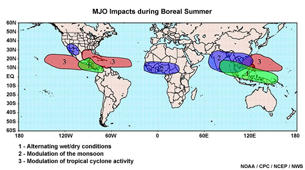
The MJO has been shown to have a range of impacts on the tropical atmosphere. In the early studies of the MJO, its passage was linked to variations in local rainfall. It has also been shown to modulate the active and break phases of the Asian–Australian and African monsoons.c Indeed, passage of the MJO has been linked to the onset, as well as active and break phases of the Australian summer monsoon system.7
A study of intraseasonal variations in tropical convection on all timescales revealed a hierarchy of convective activity36 (Fig. 4.7). The MJO provided an "envelope" of enhanced or suppressed convection. Within the active phase, synoptic-scale convection ("super cloud clusters" or SCC) were observed to propagate eastwards within the MJO envelope; thus, the SCC were propagating faster than the MJO. Consistent with their synoptic character, the SCC have spatial scale of 2000–4000 km and temporal scale of about 10 days. SCC are composed of mesoscale convective complexes (MCCs), which are quasi-circular, thunderstorm systems with spatial scales of a few hundred kilometers and temporal scale of about a day (these systems are strongly influenced by the diurnal cycle37).
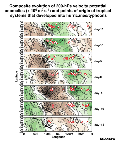
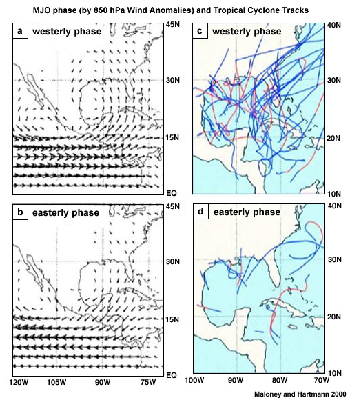
The active phase of the MJO has also been linked to increased frequency of tropical cyclones compared to the inactive phase38 (Fig. 8.68). Mesoscale convective organization in the western equatorial Pacific was shown to increase with the passage of the MJO,39,40,41,42 so that mesoscale convective complexes were evident just prior to the maximum in convection associated with the MJO passage and tropical cyclones followed (Fig. 4.8).
The MJO influence on the tropical oceans through the zonal wind anomalies results in weak zonal ocean surface stress anomalies. These wind stress anomalies have been linked to the excitation of oceanic Kelvin waves that modulate the thermocline in the equatorial Pacific.43 This is important since equatorial oceanic Kelvin waves have been hypothesized as a mechanism for triggering the El Niño/Southern Oscillation phenomenon44 (Section 4.2.1.3). Thus, it is possible that variations in the MJO may contribute to ENSO activity. Conversely, the interannual variation of the MJO may be affected by the phase of ENSO,45 although the importance of this modulation is not yet clear.12,46
The MJO influence on the tropical oceans through the zonal wind anomalies results in weak zonal ocean surface stress anomalies. These wind stress anomalies have been linked to the excitation of oceanic Kelvin waves that modulate the thermocline in the equatorial Pacific.43 This is important since equatorial oceanic Kelvin waves have been hypothesized as a mechanism for triggering the El Niño/Southern Oscillation phenomenon44 (Section 4.2.1.3). Thus, it is possible that variations in the MJO may contribute to ENSO activity. Conversely, the interannual variation of the MJO may be affected by the phase of ENSO,45 although the importance of this modulation is not yet clear.12,46
http://meted.ucar.edu/climate/beyond_mjo/index.htm
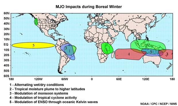
The MJO has also been hypothesized to have broader atmospheric impacts: a Rossby wave train emanates into the Northern Hemisphere midlatitudes from the Maritime Continent during passage of the active phase of the MJO through this region.7 This leads to MJO modulation of midlatitude weather, especially in the boreal winter. For example, plumes of moisture (the "Pineapple Express") flowing from MJO rainfall maxima over the central Pacific lead to heavy precipitation and floods along the west coast of the United States and Canada (Fig. 4.9).
In addition to the enhanced precipitation, winter cold air outbreaks over southern California and the southwestern deserts of North America47 are frequently timed with particular phases of the MJO.
Summary of MJO impacts globally
The impacts of the MJO on global weather patterns are summarized in Figs. 4.10a and 4.10b, which show the MJO impact on weather out to 1–3 weeks.
c The active phase of the monsoon is defined by the amplitude of the monsoon westerlies and the presence of widespread convection. The break phase has weak westerlies or easterlies and little tropical rainfall.
4.1 Sources of Intraseasonal Variability »
4.1.1 The Madden-Julian Oscillation (MJO) »
Box 4-1 Approaches for Diagnosing the MJO
Following Madden and Julian's initial studies,2,3 MJO patterns have been identified using lower and upper tropospheric winds, surface pressure, and proxies for deep convection (such as OLR, cloud top temperature, or precipitable water).
Two approaches are frequently used for diagnosing the structure and evolution of the MJO: selective filtering of the data or analysis of the data using Empirical Orthogonal Functions (EOFs).d Such diagnostics can aid in forecasting the MJO.
Filtering of the data to identify the MJO (or any other regular oscillation) requires first identifying spatial and temporal scales of the system.48,49 Two common choices for filtering are to identify the typical period of the oscillation, or its signature in wavenumber-frequency space (Fig. 4A.1). See Fig. 4.6 for an example using this approach. A brief primer on wavenumber and wave frequency is given in Box 4-2.
Filtering of the data to identify the MJO (or any other regular oscillation) requires first identifying spatial and temporal scales of the system.48,49 Two common choices for filtering are to identify the typical period of the oscillation, or its signature in wavenumber-frequency space (Fig. 4A.1). See Fig. 4.6 for an example using this approach. A brief primer on wavenumber and wave frequency is given in Box 4-2.
In recent years, EOF analysis50 (or eigen analysis or principal component analysis) has become the more popular method for identifying and predicting the MJO. Eigenanalysis identifies fundamental structures in the climate system (as represented by the fields being analyzed). The eigenvalues associated with each structure represent the strength of that structure at a given time. Hence, the spatial structure of a phenomenon with a chosen frequency or period can be identified from the periodicity of the eigenvalues. An example of prediction of the MJO based on the contribution of two eigenvectors is given in Fig. 4.13.
d Empirical Orthogonal Functions (EOFs) provide information on the way that the set of chosen variables vary most strongly together. EOFs are pure mathematical diagnostics and do not necessarily have any physical significance. Usually, however, the first few EOFs (which explain the largest percentage of the variance), are readily related to identifiable physical phenomena. http://reference.wolfram.com/mathematica/tutorial/EigenvaluesAndEigenvectors.html or similar references have more information on EOF analyses.
4.1 Sources of Intraseasonal Variability »
4.1.1 The Madden-Julian Oscillation (MJO) »
4.1.1.4 Forecasting the MJO
Forecasts of the MJO passage became available in the first few years of the 21st century. These forecasts provide guidance weeks in advance on the local wind, pressure and convection anomalies to be expected at a given location. This information contributes to an increase in general predictability of tropical weather and gives insight into the likely danger of tropical cyclone activity in regions with large MJO signatures; even where the convective signature is weak, the MJO may modulate wind shear and low-level vorticity.
Observational analysis of theoretical tropical wave structures and the MJO48 using a combination of available satellite data and global model analyses identified the evolution of the MJO structure through a complete cycle (Fig. 4.11). While the MJO can be seen in many fields without filtering, by filtering the data correctly, we can identify the MJO signal more easily (see Box 4-1).
Observational analysis of theoretical tropical wave structures and the MJO48 using a combination of available satellite data and global model analyses identified the evolution of the MJO structure through a complete cycle (Fig. 4.11). While the MJO can be seen in many fields without filtering, by filtering the data correctly, we can identify the MJO signal more easily (see Box 4-1).
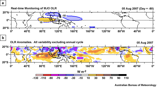
These structural analyses for phases of the MJO cycle provide the background needed to construct methods for the real-time monitoring of the MJO (e.g., Fig. 4.12).
Now we have all of the information and techniques necessary to move to the next step: MJO forecasts!
Real-time animations of the MJO diagnostics plotted in Fig. 4.12,
http://www.cawcr.gov.au/staff/mwheeler/maproom/OLR_modes/index.htm (scroll to bottom of the page)
To construct a forecast of a system with a fairly regular cycle, it is helpful to reference where you are in this cycle. For example, we refer to the "peak" and "trough" of a wave.
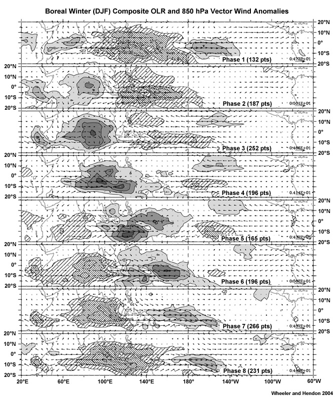
Since the MJO has a complicated spatial structure encompassing the global tropics, it is helpful to split the MJO cycle into more than two phases. A number of approaches have been used, but typically the cycle is split into either four or eight phases. One example using eight phases is plotted in Fig. 4.13.
While a number of MJO forecasts exist (Table 4.1), they all use the same basic approach of filtering observed data (including operational analyses and satellite data) based upon previously diagnosed structures for the different phases of the MJO, then constructing a statistically based forecast of the MJO evolution. The differences between the forecasts come from the choice of input data and reference structures.
While a number of MJO forecasts exist (Table 4.1), they all use the same basic approach of filtering observed data (including operational analyses and satellite data) based upon previously diagnosed structures for the different phases of the MJO, then constructing a statistically based forecast of the MJO evolution. The differences between the forecasts come from the choice of input data and reference structures.
Referring back to the phase diagram example in Fig. 4.11, we examine how RMM1 and RMM2 are constructed. The data used are near-equatorially-averaged 850 hPa zonal wind, 200 hPa zonal wind, and satellite-observed outgoing longwave radiation (OLR). Since we can see the MJO in each of these variables, we expect this analysis to give us useful information about the MJO.
Referring back to the phase diagram example in Fig. 4.11, we examine how RMM1 and RMM2 are constructed. The data used are near-equatorially-averaged 850 hPa zonal wind, 200 hPa zonal wind, and satellite-observed outgoing longwave radiation (OLR). Since we can see the MJO in each of these variables, we expect this analysis to give us useful information about the MJO.
Before we can make a forecast of the MJO, we must first filter the data used to remove both the annual cycle and interannual variability (primarily associated with ENSO). The resulting data time series now vary mostly on the intraseasonal time scale of the MJO.
Empirical Orthogonal Functions (Box 4-1) are diagnosed for the combination of these filtered data; many EOFs can be found for a given set of data, but only a few of these are likely to provide useful physical insights. The spatial structures of these EOFs are related to our initial schematic of the MJO (Fig. 4.3) in Fig. 4.14.
Empirical Orthogonal Functions (Box 4-1) are diagnosed for the combination of these filtered data; many EOFs can be found for a given set of data, but only a few of these are likely to provide useful physical insights. The spatial structures of these EOFs are related to our initial schematic of the MJO (Fig. 4.3) in Fig. 4.14.
The output of the EOF analysis is the EOFs themselves (giving structures associated with the MJO) and time series of their amplitudes. The time series of the amplitudes for the first two EOFs are RMM1 and RMM2 that are plotted in Fig. 4.12. So we see that the RMM1 and RMM2 plot tells us how OLR, 850 hPa and 200 hPa zonal wind vary together on an MJO (intraseasonal) timescale.
Note that while, the 2-D view of the MJO phases (Fig. 4.14) is very useful, it does not provide a complete representation of MJO activity, which includes a seasonal meridional variation and zonal variation related to ENSO.
| MJO Monitoring and Prediction | |
NOAA National Weather Service (NWS) Climate Prediction Center (CPC) Daily MJO Indices |
http://www.cpc.noaa.gov/products/precip/ CWlink/MJO/mjo.shtml http://www.cpc.ncep.noaa.gov/products/ precip/CWlink/MJO/index.primjo.html |
| NOAA Earth System Research Laboratory Experimental MJO Predictions |
http://www.cdc.noaa.gov/mjo/ |
Australian Bureau of Meteorology tropical variability (MJO and equatorial waves) forecasts |
http://cawcr.gov.au/staff/mwheeler/ maproom/RMM/ http://cawcr.gov.au/staff/mwheeler/ maproom/OLR_modes/ |
| MJO forecasts by Paul Roundy, State University of New York at Albany (SUNY, Albany) |
http://www.atmos.albany.edu/facstaff/ roundy/waves/ |
| MJO forecasts by Barney Love and Adrian Matthews, University of East Anglia |
http://envam1.env.uea.ac.uk/ mjo_forecast.html |
You can explore more about the MJO in the COMET webcast, The Madden-Julian
Oscillation Life Cycle presented by Dr. Roland Madden,
http://meted.ucar.edu/climate/mjo/
4.1 Sources of Intraseasonal Variability »
4.1.2 Observationally-Based Description of Equatorial Waves
In this section, we will begin by convincing ourselves that atmospheric and oceanic waves exist in the near-equatorial region, familiarizing ourselves with their basic structural characteristics. In subsequent sections, we will introduce the Shallow Water Equations and use them to understand how equatorial waves form. Finally, we will consider how convection modulates these waves and its consequences.
The theory of equatorial waves extends back to 1966 and the seminal paper of Matsuno,13 however, at the time this seminal paper was published observing systems were inadequate to diagnose these waves in the atmosphere. Subsequent work by Adrian Gill14,51 expanded this wave theory, but the question remained: "Are these theoretical waves present in the tropical atmosphere and are they important?"
In the 1980s and 1990s, technology finally enabled us to detect these waves in our atmosphere:
- Hovmöller diagrams constructed from infrared satellite imagery reveal well defined bands of cloudiness associated with westward moving disturbances in the equatorial region (~10°S-10°N) (e.g., Fig. 4.1); and
- Selective filtering of precipitable water and infrared satellite data, aimed at identifying these waves, was successful (see external links below for more information).
Some equatorial waves are observed to be coupled to convection while other waves are not, and waves that are not coupled propagate much more quickly than coupled waves.
Recent analyses of these satellite data have linked equatorial waves on the scale of 3,000–4,000 km, period range of 4–5 days, moving with speeds of ~8–10 m s-1 to initiation of tropical cyclones.52,53 As we shall see below, these characteristics suggest that Rossby or mixed Rossby-gravity waves play a role here.
NOAA ESRL, http://www.cdc.noaa.gov/map/clim/olr_modes/indiv_anim10.html
Australian BOM, http://cawcr.gov.au/staff/mwheeler/maproom/OLR_modes/
http://www.regional.org.au/au/asa/2006/concurrent/water/4734_donalda.htm
SUNY, Albany, http://www.atmos.albany.edu/facstaff/roundy/waves/
4.1 Sources of Intraseasonal Variability »
4.1.2 Observationally-Based Description of Equatorial Waves »
Box 4-2 A Quick Primer on One-Dimensional Waves
All waves result from a disturbance or instability that creates a perturbation on an initially balanced flow. Overshooting of the restoring force acting to eliminate the perturbation creates the wave oscillation. Thus, identification of the restoring force responsible for each wave type is key to understanding the formation and characteristics of that wave.
The pendulum and the weight on a string are two solid body examples often used to illustrate oscillations. An understanding of these phenomena is helpful in understanding waves. An easily observed example of an atmospheric wave is a topographically-forced gravity wave formed by moist air flowing over a ridge line in a stable atmosphere. In this case, you see lines of shallow convective clouds separated by regular clear areas. The cloud forms in the ascending part of the wave and dissipates in the descending part of the wave. Another familiar example is a surface ocean wave.
To describe a wave that varies in only one dimension, you must know its wavelength (λ), its period (τ), and its amplitude (Ao). The wavelength is the length of one complete cycle of the wave; the period is the length of time it takes for one wavelength to pass a fixed location; the amplitude is the displacement from an undisturbed surface to the peak of the wave (see Fig. 4.13). This is more generally defined as half of the displacement between the peak and the trough.
The frequency,  , of the wave can be specified in place of its period. Instead of wavelength, you could provide its wavenumber (k) given by
  .
.
An equation describing a sinusoidal wave is:
 (B4-2.1)
where Ao is the wave amplitude, x is the distance from a reference location, k is the wavenumber, ω is the frequency and t is the time since the wave was at the reference location. A more general expression for a sinusoidal wave is given by
 (B4-2.2)
where "Re" means that we are taking the real part of this expression to define the wave amplitude (which must, of course, be a measurable distance). Taking the imaginary part of this equation, "i", gives information on the growth or decay of the wave amplitude.
It is neither necessary nor possible to express every wave in terms of trigonometric functions. However, since trigonometric functions and their derivatives are familiar to all readers we will generally use these for our wave examples.
4.1 Sources of Intraseasonal Variability »
4.1.2 Observationally-Based Description of Equatorial Waves »
4.1.2.1 Kelvin Waves
Kelvin waves have long been known to fluid dynamicists interested in the atmosphere. They were first identified by William Thomson (Lord Kelvin) in the nineteenth century. Broadly speaking, Kelvin waves are large-scale waves whose structure "traps" them so that they propagate along a physical boundary such as a mountain range in the atmosphere or a coastline in the ocean.e In the tropics, each hemisphere can act as the barrier for a Kelvin wave in the opposite atmosphere, resulting in "equatorially–trapped" Kelvin waves (e.g., Fig 4.15). Kelvin waves are thought to be important for initiation of the El Niño Southern Oscillation (ENSO) phenomenon (Section 4.2.1.3) and for maintenance of the MJO.
Kelvin waves have long been known to fluid dynamicists interested in the atmosphere. They were first identified by William Thomson (Lord Kelvin) in the nineteenth century. Broadly speaking, Kelvin waves are large-scale waves whose structure "traps" them so that they propagate along a physical boundary such as a mountain range in the atmosphere or a coastline in the ocean.e In the tropics, each hemisphere can act as the barrier for a Kelvin wave in the opposite atmosphere, resulting in "equatorially-trapped" Kelvin waves (e.g., Fig 4.15). Kelvin waves are thought to be important for initiation of the El Niño Southern Oscillation (ENSO) phenomenon (Section 4.2.1.3) and for maintenance of the MJO.
Convectively-coupled atmospheric Kelvin waves (e.g., Fig. 4.15) have a typical period of 6-7 days when measured at a fixed point and phase speeds of 12-25 m s-1, while dry Kelvin waves in the lower stratosphere have phase speed of 30-60 m s-1.54,55 Kelvin waves over the Indian Ocean generally propagate more slowly (12–15 m s-1) than other regions.56 They are also slower, more frequent, and have higher amplitude when they occur in the active convective stage of the MJO.57,58
e See COMET module, Coastally Trapped Wind Reversals, http://www.meted.ucar.edu/mesoprim/ctwr/
4.1 Sources of Intraseasonal Variability »
4.1.2 Observationally-Based Description of Equatorial Waves »
4.1.2.2 Rossby Waves
The restoring force for Rossby waves is potential vorticity (PV) conservation on a varying PV field. These waves can be shown to exist even in a quiescent environment with the only variation in the PV field coming from the latitudinal variation of the Coriolis parameter—explaining why they are also known as planetary waves.f
Rossby waves were first identified by Carl Gustaf Rossby in 193959 to describe large scale quasi-geostrophic motions in the midlatitudes. These waves explain the essential elements of the evolution and spatial scales of the dominant weather systems at these higher latitudes.
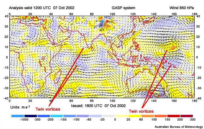
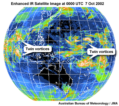
An equatorial Rossby wave can be identified in the 850 hPa tropical wind analysis pictured (Fig. 4.16) and the accompanying satellite image (Fig. 4.17). By analyzing this plot, we can gain some feeling for the spatial scale of these waves. The colors correspond to the sense of rotation associated with the wave. Hence, the east-west distance between two regions of the same color will give us the wavelength of this wave. Looking at the two regions of yellow identified north of the equator, we see that the first is located around 75°E while the second is centered near 160°E. This corresponds to a horizontal scale of almost 100° of longitude, or 10,000 km. Consideration of the two centers south of the equator confirms this scaling. This example of a Rossby wave is one of the largest (longest wavelengths) possible, since it spans about one third of the circumference of the equator. "Long" Rossby waves (waves clearly dominated by only PV conservation) typically range in size from around 4,000 to 10,000 km. The meridional distance scale of this wave is about 20° of latitude since the centers are located roughly 10° either side of the equator.
Equatorial Rossby waves are observed to have a long lifetime, on the order of days to weeks. The large waves of interest to us propagate westward with speeds on the order of 10-20 m s-1 for dry atmospheric Rossby waves, 5-7 m s-1 for convectively-coupled Rossby waves16 (and ~1 m s-1 for oceanic Rossby waves). Given that the equatorial Pacific is about 17,760 km across, an atmospheric Rossby wave would cross the Pacific in roughly 18 days and an oceanic Rossby wave would take approximately 210 days.
f Analogous waves, which have become known as "vortex Rossby waves" can be detected on the varying potential vorticity field of atmospheric vortices such as tropical cyclones (Chapter 8, Section 8.4.4.6).
4.1 Sources of Intraseasonal Variability »
4.1.2 Observationally-Based Description of Equatorial Waves »
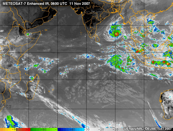
4.1.2.3 Mixed Rossby-Gravity (MRG) Waves
Mixed Rossby Gravity waves are common in the deep tropics. They force (and are forced by) clusters of thunderstorms, making these waves important for short-term weather forecasting in the tropics.
MRG identified from a variety of satellite data and numerical model analyses have longitudinal scale of 1,000-4,000 km, period range of 4-5 days and move with speeds ~8-10 m s-1. To understand why waves of this scale would succumb to variations in the mass field, we need to consider the Rossby radius of deformation, LR (Box 4-3 below, Chapter 8, Section 8.3.1). The typical Rossby radius of deformation for the tropics is on the order of thousands of kilometers.
MRG identified from a variety of satellite data and numerical model analyses have longitudinal scale of 1,000-4,000 km, period range of 4-5 days and move with speeds ~8-10 m s-1. To understand why waves of this scale would succumb to variations in the mass field, we need to consider the Rossby radius of deformation, LR (Box 4-3 below, Chapter 8, Section 8.3.1). The typical Rossby radius of deformation for the tropics is on the order of thousands of kilometers.
From this analysis, it is clear how mixed Rossby-Gravity waves earned their name: they have two competing restoring forces, PV conservation and buoyancy. Due to these dual restoring forces, MRG waves will be characterized by divergent PV centers. In the tropics such waves should be expected to be strongly modulated by moist convection (Fig. 4.18).
4.1 Sources of Intraseasonal Variability »
4.1.2 Observationally-Based Description of Equatorial Waves »
Box 4-3 Rossby Radius of Deformation, LR
The Rossby radius of deformation, LR, is a ratio between vorticity and stability. It is the horizontal length scale over which the mass (e.g., temperature, surface pressure, height) adjusts towards the wind field in geostrophic adjustment. A simple equation for the Rossby radius of deformation is
 (B4-3.1)
H is the equivalent depth and is proportional to the stability, as described in (Box 4.4).
H is the equivalent depth and is proportional to the stability, as described in (Box 4.4).
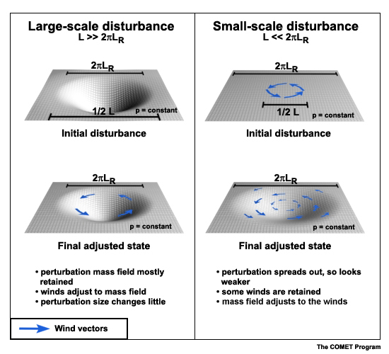
A typical equivalent depth for the free tropics is 400 m. Thus, LR ~6.3X10⁶ m or about 6300 km. Thus, a weather system with horizontal length scale, L, will evolve differently depending on the relative magnitudes of L and LR.
The Balancing Act of Geostrophic Adjustment,
http://www.meted.ucar.edu/nwp/pcu1/d_adjust/
4.1 Sources of Intraseasonal Variability »
4.1.3 Formation Mechanisms for Large-Scale Equatorial Waves
As with midlatitude theory, to gain insights into atmospheric phenomena in the tropics we resort to extensive simplifications of the Navier-Stokes equations. However, due to the weak influence of the Earth's rotation in the tropics (the Coriolis parameter, f, is zero at the equator), quasigeostrophy and other quasi-balanced flow theories are not readily applicable. Thus, flow structures in the tropics will not be as strongly constrained and should not be expected to resemble typical midlatitude patterns.
Scaling arguments show that temperature fluctuations in the tropics are very much smaller than in the midlatitudes. Applying appropriate scaling to the thermodynamic energy equation leads to
 tropics (1)
 midlatitudes (2)
Here, θ is the potential temperature, H is a typical scale height, L is a typical horizontal scale, and gravitation acceleration, g ~ 10 m s-2.
- For the tropics, reasonable values are U ~1 m s-1, and H ~104 m
- For the midlatitude regions, f ~10-4 s-1, U ~10 m s-1, L ~106 m, and H ~104 m
Substituting these values into the scaling expressions gives  values on the order of 10-3 in the tropics and 10-2 in the midlatitudes. The horizontal temperature gradients are much smaller in the tropics than in the midlatitudes so horizontal advection cannot balance the large heating observed in the regions of moist convection.
Therefore, that heating must be balanced by vertical motion. The heating in moist convection, which may be as large as 5 K day-1 or more, corresponds to strong ascent of a few cm s-1 with surrounding regions of subsidence an order of magnitude weaker.
To explore the mathematical solutions for these wave types, even in their most simplified form, we need to establish a mathematical framework. The least complex mathematical system that retains the key elements needed to define each of the three wave types is the Shallow Water Equations (see Appendix A1.1).
To explore the mathematical solutions for these wave types, even in their most simplified form, we need to establish a mathematical framework. The least complex mathematical system that retains the key elements needed to define each of the three wave types is the Shallow Water Equations (see Appendix A1.1).
We will restrict ourselves to the gravest vertical mode of those equations, extending through the depth of the troposphere. This is justified since profiles of tropical diabatic heating show maxima in the low- to mid-troposphere with weak cooling above and below. This mode has a maximum of vertical velocity in the midtroposphere and zero vertical velocity at the ground and tropopause. By continuity, these vertical variations result in horizontal velocity and pressure perturbations that have maxima at the ground and tropopause and are out of phase between these layers, and vertical motion maximum in the mid-troposphere.
Thus, lower tropospheric convergence corresponds to low surface pressure and mid-tropospheric vertical motion; associated with this is upper tropospheric divergence and a high pressure anomaly aloft. Patterns of lower tropospheric convergence (divergence) and upper tropospheric divergence (convergence) observed in the tropics are in reasonably close correspondence, reflecting this simple vertical structure for large-scale motions in the tropics as expected for regions in which convective heating dominates.
![]()
![]() Explore the dynamical response to equatorial heating in the “Two–layer model of equatorial heating”.
Explore the dynamical response to equatorial heating in the “Two–layer model of equatorial heating”.
One exception to this structure occurs in the boreal summer over the Indian Ocean region. In this season, a broad band of strong meridional flow links the easterlies in the coastal region of the east African subtropics with the monsoon westerlies over India. This warm, moist conveyor paralleling the seasonal Somali current efficiently transports moisture, fueling the Asian summer monsoon.
Lower tropospheric convergence (divergence) and upper tropospheric divergence (convergence) accompanied by with midlevel ascent (subsidence) linking these two layers imply thermally direct overturning cells. These thermally direct cells are oriented along constant latitudes (i.e. in the longitude-height plane) with ascent in the deep convection associated with strong heating over the continents.
The moist convection and associated vertical and horizontal motions generated in response to this heating explain the locations of the upward and downward branches of the east-west tropical circulation known as the Walker Circulation. Inspection of seasonal averages of the tropical windfields reveals that these Walker cells result in near cancellation of opposing zonal winds and little meridional motion. This lack of meridional motion explains the weak meridional eddy transports in the tropics. The Walker cells are not the only atmospheric response to the tropical heat sources. We now explore the sub-basin scale structures important in the tropics: waves.
Although we introduced tropical waves in terms of diabatic heating, we can solve the unforced form of the shallow water equations to derive the basic solutions for these waves. A detailed mathematical derivation for each wave type is presented in the appendices at the end of this chapter.
Although we introduced tropical waves in terms of diabatic heating, we can solve the unforced form of the shallow water equations to derive the basic solutions for these waves. A detailed mathematical derivation for each wave type is presented in the appendices at the end of this chapter.
The shallow water equations support external gravity waves that propagate at phase speed  . Further wave modes relevant to the tropics are also contained in these equations and these modes dominate the large-scale response to isolated diabatic heating maxima. We will first consider the solution for Kelvin waves, then explore the remaining wave types.
4.1 Sources of Intraseasonal Variability »
4.1.3 Formation Mechanisms for Large-Scale Equatorial Waves »
Box 4-4 Equivalent Depth
When using the shallow water equations to explore tropical atmospheric waves, the mean depth of the fluid should be set to the equivalent depth to get appropriate values for the horizontal components of motion. But how do we determine the equivalent depth?
Beginning from the three-dimensional equations for an incompressible atmosphere with constant static stability and assuming separable solutions (so that the vertical and horizontal structures of the waves can be solved separately), we can reduce this set of equations to the shallow water equations and a vertical structure equation. The vertical structure equation is typically of the form:
 (B4-4.1)
where
In this equation m is the vertical wavenumber, H is the equivalent depth, Τo is the base state (background) temperature, Hs = R Τo g-1 is the scale depth and we assumed a constant static stability,  . So the expression for the equivalent depth, H, is found from the separation constant for the horizontal and vertical structures of the wave.60,61
Using typical values for the tropics, equivalent depths for tropospheric waves in dry atmosphere with constant static stability can be shown to have typical values ranging from 10-500 m and corresponding vertical wavelengths of around 5-50 km. Consider one example: a typical deep convective event in the tropics will have maximum latent heating in the mid-troposphere (say 7 km). Assuming typical values for the lapse rate and background temperature, this gives an equivalent depth of 200 m and a vertical wavelength of 28 km.62
4.1 Sources of Intraseasonal Variability »
4.1.3 Formation Mechanisms for Large-Scale Equatorial Waves »
4.1.3.1 Kelvin Waves
Kelvin waves can be thought of as large-scale gravity waves trapped at the equator. As such, we can explore their solution by considering the unforced shallow water equations on an equatorial β-plane. We further assume that there is no meridional component of velocity. Under these assumptions, the shallow water equations reduce to
 (3)
(3) (4)
(4) (5)
(5)where  is the mean depth of the fluid, h is the perturbation on this mean fluid depth corresponding to the wave h and u is the zonal wind speed of the perturbation. This equation set is satisfied by solutions of the form
 (6)
(6)Substituting these expressions into the shallow water equations, we find expressions for co, α and 
 (7)
(7)and
 (8)
(8)Integrating this equation for  gives
gives
 (9)
(9)Here u is a constant and is the amplitude of the zonal wind perturbation associated with the Kelvin wave.
Since the phase speed, co, for the Kelvin waves does not depend on wavenumber, k, these waves are non-dispersive. As a result, all Kelvin waves having the same equivalent depth—regardless of their wavelength—will propagate eastward with the same phase speed, co.
Consideration of the mathematical form of  leads us to conclude that the negative root for co is not physically reasonable, since this would lead to a wave that grew exponentially larger as the distance away from the equator increased. Thus, the final solutions describing the Kelvin wave are
 ,
,
 (10)
(10)The meridional scale of these Kelvin waves is derived from the form of the exponential and is  This means that the wave amplitude at this distance from the equator will be reduced by e-1 ≈ 0.4 of its maximum amplitude. Thus, this meridional scale is also known as the e-folding scale of the system.
For an equivalent depth of 400 m, co is about 60 m s-1 and β = 2.3 x 10⁻¹¹ s-1, so that the meridional scale of the Kelvin wave is calculatedg to be roughly 2 x 10⁶ m or around 2000 km. This meridional length scale (corresponding to about 20° of latitude) is valid under the β–plane approximation applied since β only varies by about 6% over the 2000 km distance.h
g  , where Φ is latitude, Ω is the Earth rotation rate (7.292 x 10⁻⁵ s-1) and α is the radius of the Earth, taken to be 6.37 x 10⁶ m. Hence, at the equator, β = 2.3 x 10⁻¹¹ s-1.
h Make sure that the solution obtained does not violate any assumptions made in setting up the problem.
4.1 Sources of Intraseasonal Variability »
4.1.3 Formation Mechanisms for Large-Scale Equatorial Waves »
4.1.3.2 A General Dispersion Relation for Equatorial Waves
As discussed in the Appendix B, the dispersion relation for a wave is a mathematical expression of the relationship between the wave frequency and wavelength (usually expressed in terms of a wavenumber, k). Since  for a wave with zonal wavenumber k, the dispersion relation for the Kelvin waves is just
As discussed in the Appendix B, the dispersion relation for a wave is a mathematical expression of the relationship between the wave frequency and wavelength (usually expressed in terms of a wavenumber, k). Since for a wave with zonal wavenumber k, the dispersion relation for the Kelvin waves is just
 (11)
(11)To derive the mathematical solutions for the remaining tropical waves, we return to the complete set of shallow water equations on an equatorial β–plane,
 (12)
(12) (13)
(13) (14)
(14)Following an analogous approach to that used for the Kelvin waves (see Appendices for details), we recover a general form of the dispersion relation
 (15)
(15)where n is an integer resulting from the series solution of the wave equation and is the gravity wave phase speed solved for above. The Kelvin wave solution can be recovered from this dispersion relation for n = -1.
Further analysis of this system reveals that the meridional scale for these waves is  corresponding to a north-south e-folding distance of roughly 1 x 10⁶ m, or about 1000 km. Thus, the remaining tropical waves have smaller meridional extent than the Kelvin waves.
For n = 0, we recover mixed Rossby-gravity waves. When the wavenumber is large (wavelength is relatively small) and positive, these waves are similar in structure to eastward propagating gravity waves; for negative values of wavenumber, these waves are slowly varying and westward propagating, similar to Rossby waves.
High frequency gravity waves which propagate both east and west, and westward-propagating equatorial Rossby waves exist for solutions with n ≥ 1 in addition to the Kelvin waves, equatorial Rossby waves are an important response to isolated heating (e.g. deep convection) in the tropics.
A word of warning: these wave solutions have all been derived for a dry, incompressible atmosphere and the solutions rely on assuming the simplest vertical structure and linearizing about a state of no motion on an equatorial β–plane. While we can track waves similar to these idealized solutions in satellite data, the impacts and feedbacks of the three-dimensional wind structure, surface friction, and moisture (among others) need to be included to describe these waves quantitatively and to explain the wave structures and behaviors observed from satellite data more completely.
4.1 Sources of Intraseasonal Variability »
4.1.4 Interpreting the Mathematical Solutions for Large-Scale Equatorial Waves
Before we delve into the impacts of these modifiers of wave structures in the real atmosphere, we first consider the implications of the wave structures that we derived.
4.1 Sources of Intraseasonal Variability »
4.1.4 Interpreting the Mathematical Solutions for Large-Scale Equatorial Waves »
4.1.4.1 Kelvin Waves
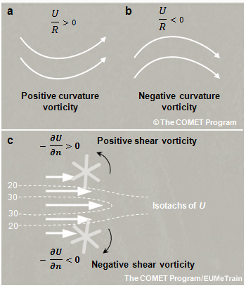
The theoretical Kelvin wave solution derived in Section 4.1.3.1 is depicted in Fig. 4.19. Only a couple of repeats of highs and lows along the equator are shown. As expected from the solutions, the pressure and zonal wind anomalies sit on the equator. These anomalies decrease away from the equator with meridional length scale of about 2000 km. There is no meridional motion associated with this wave type. The horizontal wave components combine to produce the correct sign of shear vorticity in each hemisphere; corresponding to the low or high pressure on the equator.
The theoretical Kelvin wave solution derived in Section 4.1.3.1 is depicted in Fig. 4.19. Only a couple of repeats of highs and lows along the equator are shown. As expected from the solutions, the pressure and zonal wind anomalies sit on the equator. These anomalies decrease away from the equator with meridional length scale of about 2000 km. There is no meridional motion associated with this wave type. The horizontal wave components combine to produce the correct sign of shear vorticity in each hemisphere; corresponding to the low or high pressure on the equator.
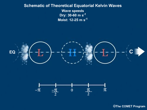
We will now use this diagram to reason through the motion resulting from this wave structure and then compare it to the theoretical solutions obtained above. Waves are maxima on the equator, so we are interested in the along–equatorial mass transports.
Following Matsuno (1966),13 we use mass advection due to wave-relative motion to explain wave propagation:
- With the low to the west of the high: Have mass divergence between them (to the east of the low) leading to pressure falls on the equator. This means falling pressure to the west of the high (east of the low), so the wave moves towards the east.
- With the high to the west of the low: Have mass convergence between them (to the east of the high) leading to pressure rises on the equator. This means rising pressure to the east of the high (west of the low), so the wave moves towards the east.
Both of these thought experiments give eastward propagating Kelvin waves.
Comparing these results with the theoretical Kelvin wave phase speed, co, derived above ( ) confirms that this eastward propagation is correct for the dry Kelvin wave. Based on this phase speed formulation, we can think of Kelvin waves as equatorially trapped, synoptic–scale gravity waves.
4.1 Sources of Intraseasonal Variability »
4.1.4 Interpreting the Mathematical Solutions for Large-Scale Equatorial Waves »
4.1.4.2 Equatorial Rossby Waves (ER)
One wavelength of a theoretical Rossby wave is depicted in Fig. 4.20. We will apply the same approach used for previous wave solutions to reason through the mass advection due to wave–relative motion to explain propagation of this wave. See that Rossby waves have the same sense of vorticity (opposite sense of rotation) either side of the equator. This results in maxima in the wind field on the equator and maxima in the mass field off–equator, so we are interested in the off–equator mass tendencies.
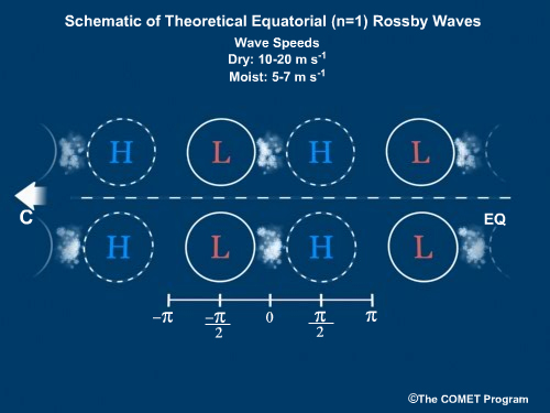
Note that since the n=1 Rossby waves have the same sense of vorticity on either side of the equator, references to high and low pressure systems are equally applicable to the Southern and Northern Hemispheres. Also, flow in the wave pattern closer to the equator is stronger than flow away from the equator.
- With high to the west of the low, mass is advected poleward, leading to pressure drops, so the low moves westward.
- With low to the west of the high, mass is advected into the region, leading to pressure rises, so the high moves westward.
Thus, in both thought experiments, the wave propagates westward.
The theoretical phase speed, c, derived by Matsuno (1966)13 is  for 1D and 2D cases respectively. This confirms that our reasoning is consistent with the dry, theoretical solution.
4.1 Sources of Intraseasonal Variability »
4.1.4 Interpreting the Mathematical Solutions for Large-Scale Equatorial Waves »
4.1.4.3 Mixed Rossby-Gravity Waves
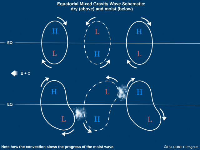
As with the other theoretical wave types discussed here, theoretical MRG waves also circle the equator, but since we only care about the very longest of these waves, less than two wavelengths are depicted in Fig. 4.21. Note that the wind field circulation straddles the equator, but the associated vorticity has different interpretation either side: the sense of rotation or shear corresponding to cyclonic vorticity to the north corresponds to anticyclonic vorticity in the Southern Hemisphere. This explains the low and high pressure pair inside one "circle" which represents the wind anomaly. Interpreting this structure can be tricky, but once again, we use mass advection due to wave-relative motion to explain wave propagation. Waves are maxima just off the equator, so we are interested in the cross-equatorial mass transports here.
We will consider the wave from the perspective of the placement of the low and high pressure centers in the Northern Hemisphere when referring to relative locations within this wave:
- With the Northern Hemisphere high to the west of the Northern Hemisphere low, mass advection across the equator (to the south) leads to pressure drops north and rises south of the equator. This means falling pressure to the west of the Northern Hemisphere low, so the wave moves towards the west.
- With the Northern Hemisphere low to the west of the Northern Hemisphere high, mass advection is northward across the equator leading to pressure rises north and falls south of the equator. This means rising pressure to the west of the Northern Hemisphere high, so once again we deduce that the wave moves towards the west.
In both of our thought experiments, the wave moves westward.
Compare this result with the theoretical phase speed, c (derived in Appendix C),
Compare this result with the theoretical phase speed, c (derived in Appendix C),
 (16)
(16)Since β > 0 everywhere on the globe and k2 > 0 for all choices of wave number and > 0 (H is the equivalent depth of the atmosphere), the square root is real (positive inside) and is greater than one. Thus, the expression inside the parentheses is negative and we once again have a negative phase speed, so the wave will propagate towards the west in agreement with the theoretical solution derived in Section 4.1.2.2.
Since β > 0 everywhere on the globe and k2 > 0 for all choices of wave number and > 0 (H is the equivalent depth of the atmosphere), the square root is real (positive inside) and is greater than one. Thus, the expression inside the parentheses is negative and we once again have a negative phase speed, so the wave will propagate towards the west in agreement with the theoretical solution derived in Section 4.1.2.2.
4.1 Sources of Intraseasonal Variability »
4.1.5 Modulation of Equatorial Waves by Moist Convection
Effects of moisture (convection) on wave propagation are based on the observational studies of Wheeler and Kiladis,16,48,55 Roundy and Frank,52 and others, and satellite images.
- For the moist Kelvin wave (e.g., Fig 4.15), have moist convergence to the west of the low, leading to deep convection here. Since the convection is to the west of an eastward moving low, and convection will generate cyclonic low-level PV, the moist convection slows the wave propagation.
- For the moist mixed Rossby–gravity wave (e.g., Fig 4.17), have moist convergence to the east of the low in each hemisphere. This gives alternating centers of convection north and south of the equator. Since the convection is to the east of a westward moving low, and convection will generate cyclonic low–level PV, the moist convection slows the wave propagation.
- When moisture is added to the equatorial Rossby wave (e.g., Fig 4.18), the moist low–level convergence to the east of ("behind") the low center can force deep convection. Deep convection generates low–level cyclonic PV, and so slows down the wave.
4.1 Sources of Intraseasonal Variability »
4.1.5 Modulation of Equatorial Waves by Moist Convection »
4.1.5.1 Impact of Convectively Coupled Equatorial Waves
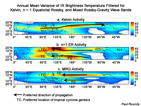
While equatorial waves propagate zonally around the entire tropical belt, their impact varies regionally. Figure 4.22 shows the spatial distribution and preferred propagation direction of equatorial waves. The geographic range of direct equatorial wave impact is limited. For example, Kelvin waves have a direct impact on convection only within about 10° of the equator (Fig 4.22a); in particular the central and eastern Pacific Ocean. Kelvin wave activity varies more by season over Africa, the Indian Ocean, and South America.63 The direct impact of n = 1 equatorial Rossby waves is strongest over the Asian monsoon and West Pacific pool regions (Fig. 4.22b) and symmetric ER waves are commonly observed over the Indian Ocean (e.g., Fig. 8.21). MRG wave activity is strongest across the western and central Pacific ITCZ regions and during the boreal summer and autumn.16
Equatorial waves contribute to tropical cyclogenesis64,52,65,66 (Fig. 4.22), especially over the Indian and west Pacific basins. See Chapter 8, Section 8.3.2.2 for more details of tropical cyclogenesis in association with ER and MRG waves.
Equatorial waves contribute to tropical cyclogenesis64,52,65,66 (Fig. 4.22), especially over the Indian and west Pacific basins. See Chapter 8, Section 8.3.2.2 for more details of tropical cyclogenesis in association with ER and MRG waves.
4.1 Sources of Intraseasonal Variability »
4.1.5 Modulation of Equatorial Waves by Moist Convection »
4.1.5.2 Monitoring and Forecasting Equatorial Waves
Real-time monitoring of equatorial waves has been conducted by NOAA since 1999 and daily plots of wave signals are available online. Other real-time monitoring sites are listed in Table 4.2. Each type of equatorial wave is identified by spatial and temporal filtering of anomalous OLR (Fig. 4.23) as well as 850 hPa and 200 hPa winds48,49,63 (see example for MJO in Section 4.1.1.4). With retrospective identification, different wave modes are easily determined for known periods of data.48 Real-time filtering of OLR assumes that future time series characteristics of OLR and other anomalies are similar to the past and uses extrapolation to determine current and future signals.49,50,56,67,68
Real-time monitoring of equatorial waves has been conducted by NOAA since 1999 and daily plots of wave signals are available online. Other real-time monitoring sites are listed in Table 4.2. Each type of equatorial wave is identified by spatial and temporal filtering of anomalous OLR (Fig. 4.23) as well as 850 hPa and 200 hPa winds48,49,63 (see example for MJO in Section 4.1.1.4). With retrospective identification, different wave modes are easily determined for known periods of data.48 Real-time filtering of OLR assumes that future time series characteristics of OLR and other anomalies are similar to the past and uses extrapolation to determine current and future signals.49,50,56,67,68
The forecast skill of these techniques varies with wave type but typically extends to about half of the period of each wave.16 So, the forecast skill for equatorial waves extends to 1-5 days; Fig. 4.24 shows observed and forecast Kelvin and n=1 ER waves. The application of these products to successful tropical forecasting has not been documented and forecasting of equatorial waves remains a challenge.
One area of potential forecast improvements from monitoring equatorial waves is intraseasonal tropical cyclone activity. Figure 4.22 shows TC formation relative to equatorial wave activity. Experimental long-range probabilistic forecasts of tropical cyclones that develop in association with convectively coupled waves and intraseasonal oscillations are being tested (Table 4.2).
| Monitoring and Prediction of Equatorial Waves | |
| NOAA/ESRL/PSD Climate Diagnostic Center, Daily OLR Modes (updated daily since 1999) |
http://www.cdc.noaa.gov/ map/clim/olr_modes/ http://www.cdc.noaa.gov/map/clim/ olr_modes/mapanim2.html |
| Australian Bureau of Meteorology Monitoring and prediction of modes of coherent tropical variability |
http://cawcr.gov.au/staff/ mwheeler/maproom/OLR_modes/ |
| Real–time evolution of modes of organized convection and forecasts, Paul Roundy, (SUNY, Albany) |
http://www.atmos.albany.edu/ facstaff/roundy/waves/ |
Experimental probability of a tropical cyclone, Dr. Paul Roundy, SUNY, Albany,
http://www.atmos.albany.edu/facstaff/roundy/tcforecast/tcforecast.html
4.2 Sources of Interannual Variability
4.2 Sources of Interannual Variability »
4.2.1 The El Niño-Southern Oscillation (ENSO)
The vital role of ocean-atmosphere interaction in tropical interannual variability is illustrated most dramatically by the El Niño-Southern Oscillation (ENSO) phenomenon. ENSO is a "coupled" atmospheric-oceanic process caused by recurring redistributions of heat and atmospheric momentum in the Equatorial Pacific.69 The zonal distribution of tropical surface heating (continental and oceanic) produces an east-west circulation pattern known as the Walker Circulation.70 ENSO perturbs the Walker Circulation and triggers major shifts in tropical rainfall patterns and deep convection, disrupting atmospheric circulations and climate across the globe.69,71,72 The extremes of ENSO, termed El Niño and La Niña, encompass a wide range of climatic conditions.71
4.2 Sources of Interannual Variability »
4.2.1 The El Niño-Southern Oscillation (ENSO) »
4.2.1.1 Description of the Walker Circulation
In addition to the meridional circulation in the Hadley Cell, the tropics also exhibit patterns of rising and sinking motion in the east-west direction. These zonal circulation cells exist because of large east-west gradients in the SST and underlying thermal structure of the Pacific and Atlantic Oceans as well as heating of the tropical continental regions. The largest region of intense precipitation occurs over the Maritime Continent. Thunderstorms and heavy rainfall are fueled by strong solar forcing, abundant evaporation from the warm Pacific and Indian Oceans, and sea-land breeze circulations that force convection on a daily basis (Chap. 5, Sect. 5.3.7.1). Latent heat release by these massive thunderstorm systems enhances rising motion and surface inflow from the east and west, thereby driving a strong circulation cell along the equator. Corresponding sinking motion occurs over the cool eastern Pacific. The large circulation cell over the Pacific was first described by meteorologist Sir Gilbert Walker.70 Large convective regions also occur with heating of tropical Africa and South America with sinking motion in between. Collectively, east-west circulation cells are referred to as the Walker Circulation (Fig. 4.25).
In addition to the meridional circulation in the Hadley Cell, the tropics also exhibit patterns of rising and sinking motion in the east-west direction. These zonal circulation cells exist because of large east-west gradients in the SST and underlying thermal structure of the Pacific and Atlantic Oceans as well as heating of the tropical continental regions. The largest region of intense precipitation occurs over the Maritime Continent. Thunderstorms and heavy rainfall are fueled by strong solar forcing, abundant evaporation from the warm Pacific and Indian Oceans, and sea-land breeze circulations that force convection on a daily basis (Chap. 5, Sect. 5.3.7.1). Latent heat release by these massive thunderstorm systems enhances rising motion and surface inflow from the east and west, thereby driving a strong circulation cell along the equator. Corresponding sinking motion occurs over the cool eastern Pacific. The large circulation cell over the Pacific was first described by meteorologist Sir Gilbert Walker.70 Large convective regions also occur with heating of tropical Africa and South America with sinking motion in between. Collectively, east-west circulation cells are referred to as the Walker Circulation (Fig. 4.25).
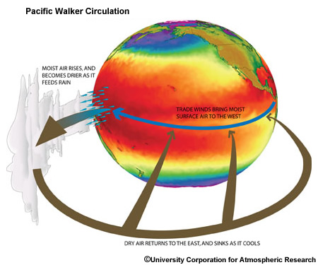
How would the global Walker Circulation change if the area of maximum anomalous warming shifted to the western Indian Ocean? Type answer in box below.
NOAA/CPC El Niño/La Niña, http://www.cpc.noaa.gov/products/analysis_monitoring/lanina/
NOAA/CPC, ENSO Cycle,
http://www.cpc.noaa.gov/products/analysis_monitoring/ensocycle/enso_cycle.shtml
NOAA/NCDC, El Niño/La Niña, http://www.ncdc.noaa.gov/oa/climate/elnino/elnino.html
4.2 Sources of Interannual Variability »
4.2.1 The El Niño-Southern Oscillation (ENSO) »
4.2.1.2 ENSO Evolution
ENSO has an irregular, two to seven-year, cycle and large areal extent (the entire tropical Pacific), and its impacts are global.73 The oceanic component of ENSO, El Niño, is characterized by weakening of the trade winds and warming of SSTs in the Equatorial Pacific (Fig. 4.26). El Niño or "Christ Child" originally referred to the appearance of warm water off the coast of Peru and Ecuador near Christmas time. It was noticed that in some years, the warming was stronger than others and disrupted local fishing. The local phenomenon has since been recognized as part of a global climate event. El Niño events typically last 9-15 months.69,74 La Niña is associated with stronger than normal trade winds and the anomalously cool SST. On average, La Niña is a less extreme anomaly than El Niño but tend to last longer, 1-3 years. El Niño to La Niña transitions occur much faster than La Niña to El Niño transitions; almost all El Niño to La Niña transitions occur in one year.74
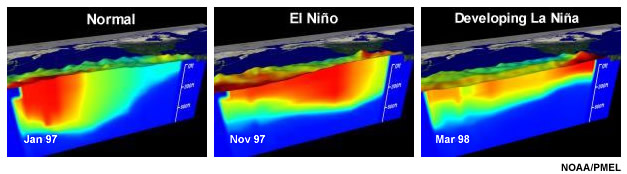
The Southern Oscillation75 is the atmospheric component of ENSO, involving a seesawing of surface pressure across the Equatorial Pacific and occurring in concert with El Niño. It is not certain whether El Niño causes the Southern Oscillation or vice–versa but an observation of an anomaly of one heralds the arrival of the other.69 Alternatively, from a coupled perspective, they both rely on and modulate each other. The Southern Oscillation Index (SOI) is the normalized difference in pressure between Darwin, Australia and Tahiti, French Polynesia, which can be calculated as
 (17)
(17)where Pdiff is the difference between the monthly mean sea level pressure of Tahiti and Darwin, Pdiffav is the long term average of Pdiff for that month (climatology).
The oscillation was noted by Sir Gilbert Walker during his quest to forecast the monsoon. The SOI is a proxy for the strength of trade winds, as pressure differences determine wind speed. The correspondence between low pressure differences (low SOI) and El Niño conditions and high pressure differences (high SOI) and La Niña is clearly demonstrated in Fig 4.27, a multi-decadal time series.
The ENSO signature is evident in the SST, mixed layer depth, upper ocean currents, and surface wind stress fields, and shift in the Walker Circulation (Fig. 4.28).
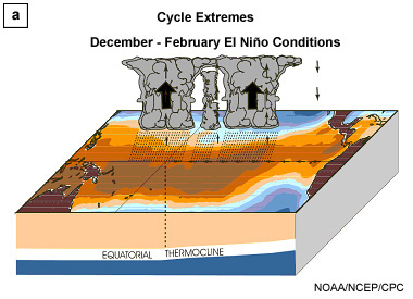
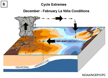
Dr. Vernon Kousky, COMET webcast, The El Niño-Southern Oscillation (ENSO) Cycle,
http://meted.ucar.edu/climate/enso/
4.2 Sources of Interannual Variability »
4.2.1 The El Niño-Southern Oscillation (ENSO) »
4.2.1.3 ENSO Theory
The ENSO signal is the strongest interannual variability in the tropics and a number of theories have been advanced for its origin and evolution.76 In 1969, Jakob Bjerknes77 noted the positive feedback between trade winds and zonal SST gradients in the equatorial Pacific. Specifically, an anomalously warm western Pacific and cold eastern Pacific lead to strong convection in the west; this convection in turn drives strong easterly trades that reinforce the SST gradient by cooling the central and eastern Pacific SST (the La Niña phase). The opposite conditions, an anomalously warm eastern Pacific, would lead to El Niño.
However, the Bjerknes theory did not explain why the ENSO anomalous conditions would end, how long they would last, or why they had their peak during the boreal winter (locked in phase to the seasonal cycle). Also, how do wind changes in the western and central Pacific lead to changes in sea surface heights in the eastern Pacific? There is also the question of whether the atmosphere-ocean feedbacks are stable or unstable. ENSO can remain in the same state for extended periods although these feedbacks are present.78
El Niño is characterized by anomalous westerly winds. Westerly anomalies form when trade winds weaken or westerly winds develop with large-scale phenomena such as the MJO.79,80 A westerly wind burst is a synoptic-scale disturbance comprised of strong westerly winds near the equator. Westerly wind bursts are identified by three conditions: surface zonal winds anomalies of 5 m s-1 or greater; the wind anomalies extend over at least 10° longitude; anomalies last for at least 2 days, and the center longitudes of the two continuous days is within 7.5° of each other.80
If the trade winds weaken, an initial westerly wind stress anomaly in the central Pacific causes the generation of an eastward propagating and downwelling oceanic Kelvin wave.81,82 The downwelling wave deepens the thermocline in the west and heightens it in the east. Oceanic Kelvin waves are trapped along the equator (e.g., Fig. 4.29) and are, typically, 5-10 cm high, hundreds of kilometers wide, a few degrees warmer than surrounding waters. They have phase speeds of 2-3 m s-1 and cross the Pacific in about 3 months.83
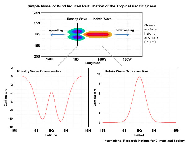
Equatorial Kelvin wave model, Dr. Peter Bannon, Pennsylvania State University,
http://www.ems.psu.edu/~bannon/mpegs/eqkel.mpg
* Delayed Oscillator Theory
One current theory, that apparently fits many observations of ENSO, is the delayed-oscillator theory postulated by scientists in the late 1980s.84,85 These studies used coupled atmosphere-ocean dynamics, including convective heating in the atmosphere, explicit representation of the surface-layer dynamics and thermodynamics to determine the SST, and linear shallow-water dynamics along the equator (Section 4.1.3, Box 4-5). These coupled models show that a growing ENSO carries with it the seeds of its own demise.
One current theory, that apparently fits many observations of ENSO, is the delayed-oscillator theory postulated by scientists in the late 1980s.84,85 These studies used coupled atmosphere-ocean dynamics, including convective heating in the atmosphere, explicit representation of the surface-layer dynamics and thermodynamics to determine the SST, and linear shallow-water dynamics along the equator (Section 4.1.3, Box 4-5). These coupled models show that a growing ENSO carries with it the seeds of its own demise.
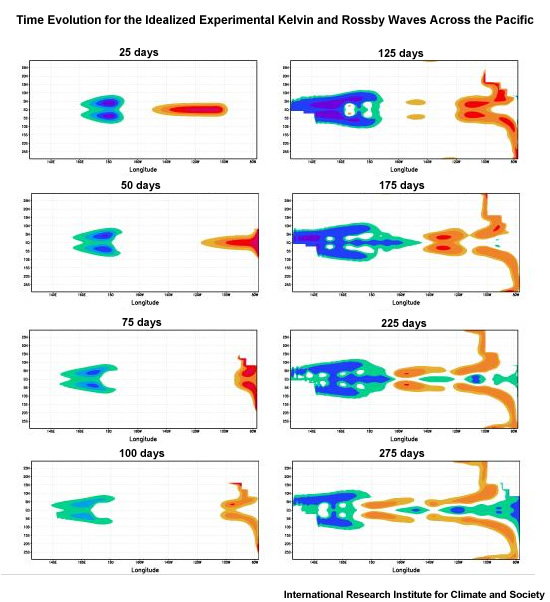
When trade winds falter and westerly wind anomalies persist for long months, strong Kelvin waves move east across the equator (e.g., Fig. 4.31). Coincident with the eastward-moving Kelvin wave are westward-moving Rossby waves (Fig. 4.29). The series of Kelvin waves leads to anomalous warming of the eastern and central Pacific. At the eastern boundary (South America) the eastward-propagating Kelvin waves reflect in the form of upwelling Rossby waves that spread out along the coast and move westward on either side of the equator (75-100 days in Fig. 4.30). The westward-propagating Rossby waves within 10 degrees of the equator are the fastest of the Rossby modes and create a shallower thermocline to the west. The slower-moving Rossby waves reflect off the western boundary (the Maritime continent) and propagate eastward as upwelling Kelvin waves that raise the thermocline in the eastern ocean (125-175 days in Fig 4.30). An oceanic Rossby wave takes approximately eight months to cross the Pacific. Therefore the oscillatory cycle will reverse the initial SST warming about six months after its onset. The delayed-oscillator theory can explain the tendency for cold anomalies to follow warm anomalies and the typical time scale of an El Niño event. However, the delayed oscillator theory does not explain the termination of cold events. For that phase of ENSO, the observed Kelvin wave amplitude and the wind stress are poorly correlated relative to that expected from the delayed oscillator theory; ENSO is less periodic than this theory suggests.86,87
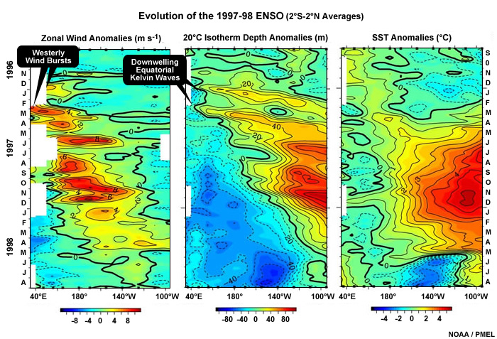
* Linear Stochastic Theory
The linear stochastic theory suggests that the development of El Niño and its demise occur in partial response to modulation of higher-latitude patterns by the global ENSO pattern in atmospheric moist deep convection.91 In essence, the coupled ocean-atmosphere system is stable and ENSO events would not occur without external random forcing that cause SST growth or decay.76
* Recharge/discharge Theory
The recharge/discharge theory92 postulates that, prior to El Niño, heat content builds up in the equatorial region; the heat is then "discharged" eastward and poleward during El Niño. Transport below the Ekman layer is the key to recharge and discharge (Fig. 4.32).
 n and McPhaden 2002)93
* Western Pacific Oscillator Theory
The Western Pacific Oscillator theory94 (Fig. 4.33) begins with condensation heating in the west central Pacific, which induces twin off-equatorial cyclones and westerly wind anomalies at the equator. The anomalous wind stress deepens the thermocline and increases the SST in the east Pacific. Positive feedback between wind stress and SST leads to growth of the anomaly. Meanwhile the pair of cyclones raises the thermocline, so that SST decreases and sea level pressure increases off the equator in the west Pacific. Anomalous high pressure induces easterly wind anomalies which causes upwelling and cooling. The cooling spreads eastwards and provides a negative feedback, thereby creating an oscillating coupled ocean-atmospheric system. Unlike the delayed oscillator theory, this theory does not require wave reflection for the coupled ocean-atmosphere system to oscillate.
* Advective-Reflective Oscillator
The Advective-Reflective Oscillator theory95 proposes that westerly wind anomalies induce anomalous eastward zonal currents. El Niño results from positive feedback of zonal currents that advects the western Pacific warm pool toward the east. The warm pool would be pushed back towards the west by zonal currents associated with wave reflection at the western and eastern boundaries, and by convergence of the mean zonal current at the eastern boundary of the Pacific.
* The Unified Oscillator
The Unified Oscillator Theory96 tries to combine the earlier oscillation mechanisms. It formulates the interactions of anomalies of sea surface temperatures in the eastern Pacific, zonal wind stress in the central and western equatorial Pacific, and thermocline depth in the off-equatorial western Pacific.
Fundamentally, the background mode of the coupled ocean-atmosphere system of the Pacific varies with the annual cycle and decadal influences. ENSO is dependent on the ocean memory and its dynamical adjustment time.
4.2 Sources of Interannual Variability »
4.2.1 The El Niño-Southern Oscillation (ENSO) »
Box 4 - 5 ENSO Behavior and Coupled Ocean-Atmosphere Models
As described earlier, the ocean is coupled to the atmosphere through wind stress anomalies,77 while winds are driven by elevated latent heat release through convection14 and SST gradients.88 The coupling can be expressed as,
 (B4-5.1)
where τ is the coupled zonal wind stress, Τ is the SST, and μ is the coupling coefficient that signifies the strength of the coupling.
Using the delayed oscillator theory as an example, the ENSO mode can be described by a differential–delay equation.
 (B4-5.2)
where Τ is the SST anomaly in the eastern equatorial Pacific, t is time, c is the sum of all processes that induce local changes in τ (such as horizontal advection, thermal damping, anomalous upwelling and changes in local subsurface structure), b accounts for reflection of Rossby waves into Kelvin waves at the western boundary, and τ is the delay (lag) due to this reflection. The term, cΤ, represents the positive feedback, while bΤ (t - τ) is a delayed negative feedback representing adjustment processes in the ocean.
A broad spectrum of models has been used to understand and predict ENSO. The earliest coupled ENSO models were parameterized versions of Equation (B4-5.2).85,89 Coupled ocean-atmosphere models are classified as simple models, intermediate models, or hybrid coupled models, and coupled general circulation models. Simple atmospheric models are based on modified shallow water equations,
 (B4-5.3)
 (B4-5.4)
 (B4-5.5)
where is the mean depth of the fluid, h is the perturbation on this mean fluid depth corresponding to the wave, u and v are the perturbation wind speed components; g is acceleration due to gravity; and A represents frictional terms.
Simple tropical ocean models are also based on the shallow water equations, and include upwelling and local subsurface effects.90 For example,
 (B4-5.6)
 (B4-5.7)
 (B4-5.8)
 (B4-5.9)
where h is the layer depth (of mean value H); u and v are the zonal (x) and meridional (y) velocities, β is the derivative of the Coriolis parameter with respect to latitude, τx and τy are the zonal and meridional wind-stresses, g' is reduced gravity, and ε is a damping coefficient for a crude representation of momentum and heat mixing, and KΤ is a coefficient that depends on the mean state averaged over a box in the equatorial Pacific.
Developing a Theory for ENSO, Lecture by Dr. David Battisti,
http://www.asp.ucar.edu/colloquium/2000/Lectures/battisti1.html
4.2 Sources of Interannual Variability »
4.2.1 The El Niño-Southern Oscillation (ENSO) »
4.2.1.4 Monitoring ENSO Evolution
The amplitude of the ENSO anomaly can vary greatly.71,97,98 Several variables are measured in order to understand the relative strengths of ENSO events when compared to each other and with the neutral state. Variables routinely monitored include SST fluctuations, surface pressure shifts, trade wind intensity variations, and many other elements, using direct observations as well as remote sensing techniques.73,99,100
In the past, in situ measurements of ocean surface temperatures were obtained primarily from ship observations in different regions of the equatorial Pacific (Fig. 4.34). Data were available only sporadically because of reliance on the chance proximity of ships and the whims of their crews. Today, real-time data are obtained from a number of sources, including an advanced array of moored ocean buoys stretching across the equatorial Pacific (Fig. 4.35a).
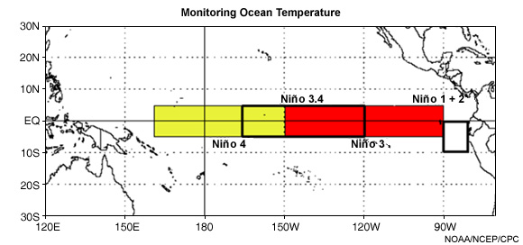
The Tropical Atmosphere Ocean (TAO)/TRITON Buoy Array
The Tropical Atmosphere Ocean (TAO)/TRITON buoy array,99 is a multi-national collaboration between United States, Japan, Korea, Taiwan, and France, and consists of nearly 70 moored buoys (Fig. 4.35). The buoys measure a full complement of atmospheric elements including surface winds, sea surface temperature, currents, ambient air temperature, and humidity, and transmit the data back to terrestrial data receivers. Availability of data in real-time from the TAO/TRITON array has proven to be an enormous benefit for detecting and predicting climate variations in the Pacific. Additional data come from satellites, ships, and the Trans Pacific Profiler Network, a network of very high frequency wind profilers established in 1984 (Fig.4.36).
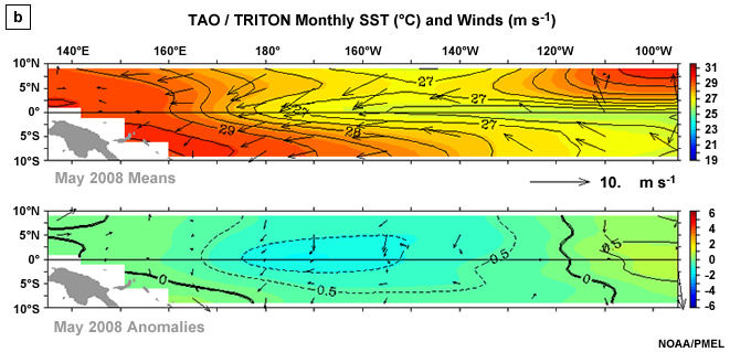
Arrays of deep ocean buoys were also established in the tropical Indian and Atlantic Oceans (Fig. 4.36). The Prediction and Research moored Array in The Atlantic (PIRATA)101,102 was established in 1997 by France, Brazil, and the United States to investigate tropical variability and climate prediction in the Atlantic, Africa, and the Americas. The Research moored Array for African-Asian-Australian Monsoon Analysis and Prediction (RAMA),102 was established with support from Japan, India, the United States, Indonesia, China, and France. As of May 2008, 18 of 46 planned mooring sites were instrumented to provide data for advanced monsoon research and climate forecasting.
TAO Array Upper ocean temperature and dynamic height for 60 months,
http://www.pmel.noaa.gov/tao/jsdisplay/plots/gifani/t-dyn.gif (9MB)
Real-time data from the TAO array, http://www.pmel.noaa.gov/tao/jsdisplay/
PIRATA Home, http://www.pmel.noaa.gov/pirata/
4.2 Sources of Interannual Variability »
4.2.1 The El Niño-Southern Oscillation (ENSO) »
4.2.1.5 Indices used to Monitor ENSO Evolution
The NIÑO 3.4 region (Fig. 4.34) is considered to be most suitable for monitoring climate variability on global scales, as SST variability here signals the strongest effect on shifting precipitation patterns from the west to the central Pacific.103 It has also been observed that prognostic numerical weather models exhibit the highest skill when initializing with data from this region.104
* The Oceanic NIÑO Index (ONI)
The Oceanic NIÑO Index (ONI) is defined as the three-month average of sea surface temperature departures from normal in the NIÑO 3.4 region of the Pacific.100,105 The average values are based on homogeneous, historical SST analyses, the Extended Reconstructed SST.106 El Niño periods are characterized by a positive ONI greater than or equal to +0.5°C. La Niña periods are characterized by a negative ONI less than or equal to -0.5°C. To be classified as a full-fledged El Niño or La Niña episode these thresholds must be exceeded for at least five consecutive months.
* Japanese Meteorological Agency (JMA) Index
The JMA index is defined by the 5-month running average of SST anomalies over the tropical Pacific (4°S–4°N, 150°W–90°W).107 A JMA index warm phase occurs when the 5-month running average of SST anomalies is greater than 0.5°C for at least six consecutive months including October to December. A cold phase occurs when SST anomalies are less than 0.5°C for at least six consecutive months including October to December. According to the JMA, an ENSO year begins in the October when the warm or cold phase forms until the following September.
* Tahiti-Darwin SOI
The most commonly used atmospheric index is the Tahiti-Darwin SOI described previously (Section 4.2.1.2).
The most commonly used atmospheric index is the Tahiti-Darwin SOI described previously (Section 4.2.1.2).
* Equatorial SOI
The equatorial SOI is defined as the standardized anomaly of the difference between the area-average monthly sea level pressure in an area of the eastern Pacific (80°W-130°W, 5°N-5°S) and an area over Indonesia (90°E-140°E, 5°N-5°S). The Equatorial SOI tracks closely with the Tahiti-Darwin SOI but with varying amplitude.
* Multivariate ENSO Index (MEI)
The Multivariate ENSO Index (MEI)97,98 is based on the six main observed variables over the tropical Pacific: sea-level pressure, zonal and meridional components of the surface wind, sea surface temperature, surface air temperature, and total cloudiness fraction of the sky. The MEI is computed over bimonthly seasons (Dec-Jan, Jan-Feb, …, Nov-Dec) for each variable (Fig. 4.38). First, the individual variable fields are filtered spatially into clusters. Then the MEI is calculated as the first unrotated Principal Component of the six fields combined.
Various low-level wind indices, upper-level wind indices, and OLR anomalies are also used to monitor ENSO evolution. It should be noted that no single ENSO index is capable of representing all ENSO variability; as many as eight modes of variability are needed to fully characterize ENSO development.91 The various ENSO indices serve a useful purpose for communicating the general state of ENSO to decision makers and the general public, e.g., the NCEP ENSO alert system provides El Niño/La Niña watches, advisories, and intensity classifications.100 However, the tropical Pacific can exhibit simultaneously characteristics of El Niño and La Niña (e.g., the east Pacific can be anomalously warm while the central Pacific is cold, as observed in the boreal summer of 2008).
http://www.bom.gov.au/climate/tropnote/tropnote.shtml
Multivariate ENSO Index, http://www.cdc.noaa.gov/people/klaus.wolter/MEI/
Equatorial SOI time series, IRI,
http://ingrid.ldeo.columbia.edu/maproom/.ENSO/.Time_Series/Equatorial_SOI.html
4.2 Sources of Interannual Variability »
4.2.1 The El Niño-Southern Oscillation (ENSO) »
4.2.1.6 Comparing El Niño and La Niña Atmospheric and Oceanic Anomalies
The first composite of El Niño SST anomalies and surface wind fields was developed by Rasmusson and Carpenter in 1982.108 The extremely warm ocean mean and anomalous SSTs during a strong El Niño is a dramatic contrast to the relatively cool conditions during a strong La Niña (Fig. 4.39). However, the two conditions are not mirror images. Anomalous warming spreads out from the eastern and central Pacific while maximum anomalous cooling is centered in the central Pacific and extends toward the northeastern Pacific (Fig. 4.39, lower panels). A similar pattern is evident in composite plots; the La Niña maximum is west of the El Niño maximum (Fig. 4.40a).
The corresponding pressure anomalies are also different. The low associated with El Niño is more confined to the eastern Pacific, while the La Niña high pressure anomaly extends farther west (Fig. 4.40b). The zonal and meridional wind anomaly plots are similar for both extremes except that the amplitudes are larger in the El Niño composite and the zonal wind anomalies are more farther west during La Niña (Fig. 4.41).
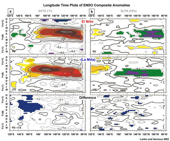
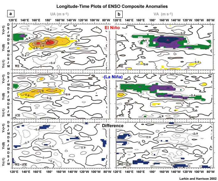
While composites provide a general pattern of anomalies, it is important to note that no two El Niños or La Niñas are the same. ENSO anomalies vary in amplitude (Fig. 4.42) and extent (Fig. 4.43). The strength and distribution of the ocean warming determines the atmospheric response and the extent of the climate impacts. For example, the 1986-87 El Niño had weak warming in the central equatorial Pacific and the impact on the atmosphere was also weak.

4.2 Sources of Interannual Variability »
4.2.1 The El Niño-Southern Oscillation (ENSO) »
4.2.1.7 Climate Impacts Related to ENSO
As expected, most of the climate impacts of ENSO are felt in the equatorial Pacific and surrounding regions,109,110 (Fig. 4.44). Most notable is heavy precipitation and flooding in northwestern South America, especially in Peru, Ecuador, and Colombia during December to February of El Niño. Effects also include loss of fish and clam populations,111 which are important to the economy and food supply of the region. Meanwhile, in Australia and the Maritime continent, the same period is marked by drought.112 Along with the drought comes wildfires and widespread smoke, which reduces visibility and leads to an increase in respiratory illnesses. El Niño has its strongest and most widespread impacts during the boreal winter.113,114 During the austral winter, El Niño impacts are weaker and felt mostly in the Southern Hemisphere.
Although precipitation effects do increase as the intensity of El Niño and La Niña increases, events of similar intensity (as defined by Niño 3.4 anomalies) do not produce effects of the same magnitude. The largest precipitation effects, as measured by the fractional area of tropical precipitation extremes, are observed during the strongest El Niño episodes (e.g., 1982/83 and 1997/98).100
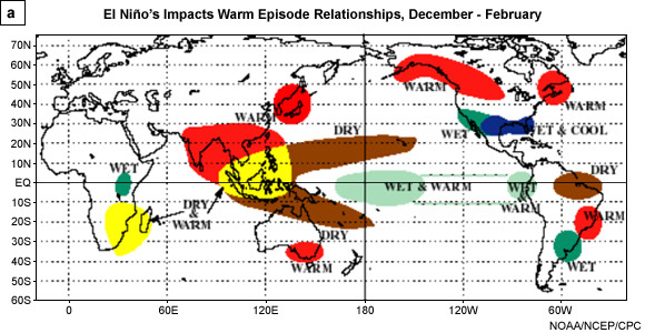
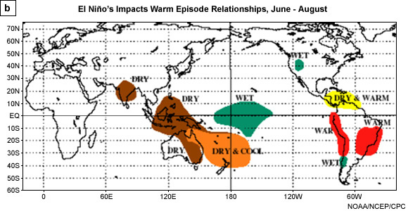
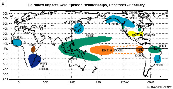
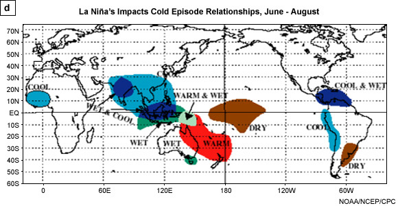
The ENSO extremes lead to a displacement or disruption of the jet streams across North America.115,116 During a warm episode (El Niño) winter in the Northern Hemisphere, the subtropical jet stream shifts southward, displaces storm tracks to the southern US, enhances moisture flow from the Pacific, and leads to heavy rainfall across the southern US, Central America, and the Caribbean (Fig. 4.44). In the United States, ENSO is known to influence temperature and precipitation distributions;115,116,117,118,119 frequency of generation of cyclones in the Gulf of Mexico;120 cloud cover;121 and a wide range of meteorological hazards including tornadoes,122,123,124 hurricanes,125,126 (Fig. 4.45) lightning,127 (Fig. 4.46) snow pack,128 and wildfires.129,130 Beneficial impacts of El Niño include warmer winters in Canada and the northern US and fewer hurricanes in the Atlantic. About 90% of the US has at least one statistically significant historical weather association with the intense 1997-98 El Niño.131
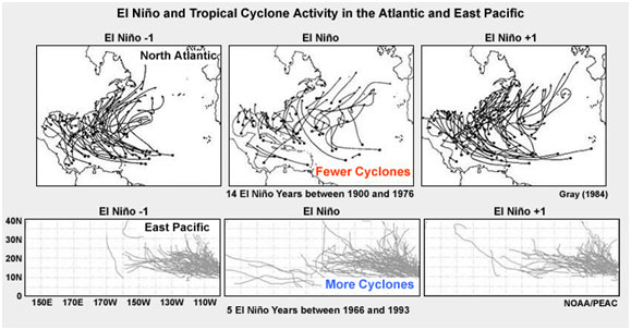
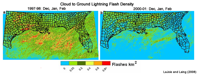
During La Niña, the probability of a hurricane making landfall is increased across the entire Caribbean,132 while El Niño periods have fewer hurricanes125 (Fig. 4.45). The increase during the cold phase is due to more easterly upper-level wind, thereby favoring the formation of hurricanes in the deep Tropics while the warm phase is marked by strong upper-level westerly winds125 and increase in anticyclonic vorticity at in the lower troposphere.133 ENSO impacts are not symmetric; the influence of El Niño is strong over the northern Caribbean and weak over the east and west Caribbean while hurricane landfall probabilities increase across the entire region during La Niña.
Impacts of ENSO vary spatially and temporally. For example, over Indonesia ENSO impacts on precipitation reaches a maximum during August and September. The impact is felt first in the east and moves westward until the peak in August.112 While the global map of ENSO impacts shows a large area of influence over Central America and the Caribbean (Fig. 4.44), the regional effects are much more complex. While La Niña is generally more wet and El Niño drier, abnormally dry and abnormally wet periods occur during both El Niño and La Niña episodes and the regions of the extremes are not always collocated (Fig. 4.47).
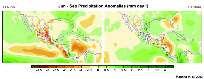
Global Precipitation Anomalies, January 1997 to February 1998
Evolution of the 1997-98 ENSO, http://www.meted.ucar.edu/afwa/climo/stats/3_5_1_pop.htm
Extratropical Anomalies: Response to Tropical Anomalies
ENSO impacts in the extratropics occur because some regions are particularly sensitive to variations in tropical heating associated with ENSO and the MJO.135 Tropical influences are felt preferentially in exit regions of the midlatitude jets.114 Heating over the Maritime Continent and nearby ocean has a great impact on the extratropics through Rossby wave trains that modulate the Pacific-North American (PNA)136 synoptic pattern.
The PNA depicts variability in the mid-tropospheric flow over North America and the North Pacific and it is most pronounced during winter. A positive PNA has a strong wave like pattern across the continent while a negative PNA has a more zonal pattern. The PNA is strongly correlated with ENSO, which leads the PNA anomaly, suggesting that ENSO influences the interannual variability of the PNA.137,114 Both are marked by shifting positions of the polar and subtropical jets and, consequently, winter cyclone tracks across North America, Central America, and the Caribbean. Figure 4.48 show the dramatic difference in the PNA pattern between strong El Niño and strong La Niña events.138
Interannual variability in the Atlantic is more closely related to the North Atlantic Oscillation (NAO) than ENSO. The NAO which is defined by pressure differences between the Azores and Iceland, has its strongest influence at high latitudes, while the PNA influences the midlatitudes. Subtropical climates are sensitive to the position of the Subtropical Jet and the Atlantic ridge, which are controlled by the tropical ENSO and the extratropical PNA and NAO.
Attributing ENSO Impacts
Since the strong 1982–83 El Niño and the recognition of its relationship to global impacts (Fig. 4.49), the popular media has tried to link nearly all climate impacts to ENSO. While the ENSO signal is the most significant extreme of tropical interannual variability, it is not the only cause of seasonal and interannual variability. Other circulation patterns influence regional climate, we should be cautious in attributing various impacts to ENSO. Before an event can be classified as an ENSO influenced event, it is helpful to ask the following questions suggested by the IRI:
- What is an ENSO impact, and what is not?
- How consistently do the impacts occur during ENSO events?
- How and why do the impacts vary from one event to another?
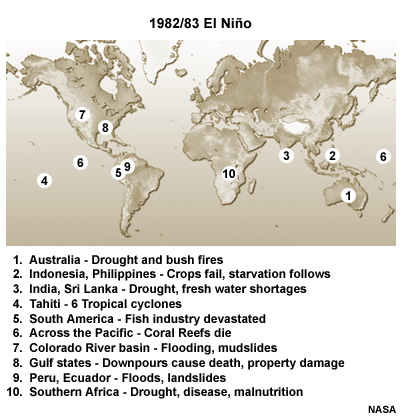
Figure 4.50 presents an illustration of the problems of attributing particular impacts to ENSO. In this instance, there are several steps between attributing a more intense jet stream to El Niño and CO poisoning among residents of poorly ventilated houses who used gas heaters after an ice storm. Each step has a level of uncertainty in attribution.
Another potentially highly relevant question to consider is how ENSO modulates the behaviors of higher-frequency patterns—such modulation effects would not correlate linearly with ENSO, but would still be associated with it.
Review of Causes and Consequences of Cold Events: A La Niña Summit,
http://ccb.colorado.edu/lanina/summary.html
NOAA, Economic implications of an El Niño, http://www.magazine.noaa.gov/stories/mag24.htm
Florida State University, El Niño cartoons, http://www.coaps.fsu.edu/lib/climatoons/
4.2 Sources of Interannual Variability »
4.2.1 The El Niño-Southern Oscillation (ENSO) »
4.2.1.8 Forecasting ENSO
In response to the 1982–83 El Niño, monitoring and modeling of ENSO expanded rapidly. One of the early achievements was the successful forecast of the 1986–87 El Niño, with lead times of 3 to 9 months by Mark Cane and Steve Zebiak at the Lamont–Doherty Geological Observatory, Columbia University.139,140 Established coupled ocean-atmosphere models now give encouraging predictions of ENSO with a 1–year lead. However, they tend to underestimate the amplitude of the interannual variability of SST141 and they have less skill between boreal winter and early spring.140 For example, while several dynamical and statistical models predicted anomalously warm SSTs for 1997, the trends were weak and too slow.140,142 The models failed to forecast the onset of the extremely strong 1997–98 El Niño during the early spring. The model forecasts improved after April–May 1997,143 many because they were initialized with the highly anomalous atmospheric and oceanic observations.
What do ENSO models predict? They predict the sea surface temperature in the equatorial Pacific. Two types of models are used, “dynamical” and “statistical” models. Dynamical models use the physical laws that govern the behavior of the atmosphere and the ocean to predict their future state. For example, Newton's laws of motion are used to predict wind velocity. Mathematical representations of the physical laws are converted into computer programs. Increasing computational power facilitates the representation of more complex behaviors of the atmosphere and ocean in dynamical models. Statistical models use past observations to predict the future. A long period of record (30–50 years) is examined for trends, extremes, and relationships between ENSO related variables. For example, a basic statistical model would be a simple regression of westerly wind anomalies and SSTs for different regions of the equatorial Pacific. More complex statistical models use neural networks in which the model is trained to recognize precursor events and predict the probability of different ENSO conditions.
In general, statistical models have greater forecast skill for short times (less than six months) but are less accurate for longer lead times. Dynamical models have seen improvements in their skill with the addition of various schemes by which real data is assimilated into the simulations. A look at current dynamical model forecast SST anomalies show that they have a wider spread of forecast values with roughly equal numbers having cold and warm biases (Fig 4.51a). While statistical models have a smaller spread, they tend to have persistently warm or persistently cold biased forecasts (Fig. 4.51b).
Improvements in the seasonal forecast skill will benefit decision makers because the impacts of ENSO vary geographically and seasonally (Fig. 4.52). For example, when the El Niño alert was given in May 1997, northwestern South America had only about a month to prepare for their period of greatest impact while other regions had a longer lead time to their period of maximum impact.
While forecast models continue to improve, ENSO predictability is limited by a number of factors. Forecasts are more difficult from January to April (referred to as the “spring predictability barrier”), which means that an El Niño is underway before the models will forecast its appearance.140,142 Stochastic processes, external forcing by weather events (white noise), help to maintain ENSO variability. ENSO is also modulated by decadal fluctuations such as the Pacific Decadal Oscillation (Section 4.3).144 The dynamical processes that contribute to the “spring predictability barrier” are not understood but the model forecast skill improves in some decades and decreases in others. Table 4.3 presents a list of ENSO forecast sites.
While forecast models continue to improve, ENSO predictability is limited by a number of factors. Forecasts are more difficult from January to April (referred to as the “spring predictability barrier”), which means that an El Niño is underway before the models will forecast its appearance.140,142 Stochastic processes, external forcing by weather events (white noise), help to maintain ENSO variability. ENSO is also modulated by decadal fluctuations such as the Pacific Decadal Oscillation (Section 4.3).144 The dynamical processes that contribute to the “spring predictability barrier” are not understood but the model forecast skill improves in some decades and decreases in others. Table 4.3 presents a list of ENSO forecast sites.
Imagine how you might use the ENSO diagnoses and predictions if you were:
- A national fire response coordinator in Australia
- A leader of an agricultural cooperative in the Philippines
- A water resource manager in Venezuela
- An emergency/disaster preparedness manager in Southern California
- A minister of road works and transportation in Ecuador
- A fisherman in Peru
- An executive of a heating gas company in western Canada
- A health official with responsibilities for respiratory illnesses in Indonesia
- A severe weather forecaster in the southeastern US
| ENSO / Tropical Pacific SST Predictions | |
| Latest El Niño/La Niña Advisory National Center for Environmental Prediction (NCEP) |
http://www.cpc.ncep.noaa.gov/ products/analysis_monitoring/ enso_advisory/index.shtml |
| Official NWS forecasts and outlooks for the US NOAA/NWS Climate Prediction Center |
http://www.cpc.ncep.noaa.gov/ products/predictions/ |
| Forecast Forum–technical discussion of forecasts from different centers |
http://www.cpc.ncep.noaa.gov/ products/CDB/Forecast/forecast.shtml |
| ENSO predictions NOAA PMEL |
http://www.pmel.noaa.gov/tao/elnino/ forecasts.html#enso |
| Summary of ENSO Model Forecasts International Research Institute for Climate and Society (IRI) |
http://iri.columbia.edu/climate/ENSO/ currentinfo/SST_table.html |
| Experimental Long-Lead Forecast Bulletin Center for Ocean-Land-Atmosphere Studies (COLA) |
http://www.iges.org/ellfb/ |
| El Niño and other Experimental Results Predictive Ocean Atmosphere Model for Australia |
http://poama.bom.gov.au/ |
| CFS Forecast Seasonal Climate Anomalies NCEP Environmental Global Climate & Weather Modeling Branch |
http://www.cpc.ncep.noaa.gov/ products/ analysis_monitoring/ lanina/ensoforecast.shtml |
| Experimental El Niño Forecast Scripps Institution of Oceanography / Max Planck Institute for Meteorology Prediction model |
http://meteora.ucsd.edu/~pierce/ elnino/elnino.html |
| Seasonal Forecasts NOAA Earth System Research Laboratory |
http://www.cdc.noaa.gov/seasonalfcsts/ |
| Seasonal Forecasts for the tropics European Centre for Medium-Range Weather Forecasts (ECMWF) |
http://www.ecmwf.int/products/forecasts/ seasonal/introduction/ |
| Equatorial Pacific SSTA forecasts Lamont-Doherty Earth Observatory of Climate Modeling Group, Columbia University |
http://rainbow.ldgo.columbia.edu/ %7Edchen/forecast.html |
| Pacific ENSO Update University of Hawaii |
http://www.prh.noaa.gov/ peac/update.php |
| SST forecasts from the neural network model Climate Prediction Group, University of British Columbia |
http://www.ocgy.ubc.ca/projects/ clim.pred/climate.html |
4.2 Sources of Interannual Variability »
4.2.2 The Quasi Biennial Oscillation (QBO)
The Quasi-Biennial Oscillation (QBO) is an oscillation that is most easily seen in the zonal winds in the lower equatorial stratosphere (typically measured around 30-50 hPa). The winds oscillate with a roughly two-year cycle from easterly to westerly and back (Fig. 4.53). These oscillations change the vertical wind shear at the top of the troposphere. The phase and magnitude of QBO have influenced the frequency of North Atlantic tropical cyclones.125,133
We will briefly review the history of QBO research, the QBO structure, then look at the impacts of the QBO on other atmospheric phenomena and finally explore a simple theory for its variation.
QBO 30 hPa zonal wind index for January 1953–September 2001
http://www.jisao.washington.edu/data_sets/qbo/index.my_page.html
4.2 Sources of Interannual Variability »
4.2.2 The Quasi Biennial Oscillation (QBO) »
4.2.2.1 The Discovery of the QBO
In 1908, westerly winds were observed at about 15 km (100–150 hPa) using weather balloons launched near Lake Victoria in Africa. These westerly winds provided a conundrum: dust from the Krakatau volcano (6°S, 105°E) eruption on August 27th, 1883 had traveled in a westward direction, taking 13 days to circle the equator. To resolve this conundrum, the notion of "Krakatoa easterlies" at around 30 km (10 hPa) and "Berson westerlies" around 20 km (50 hPa) was proposed.145
Improved insight on the behavior of the lower stratospheric winds came in 1961, when Reed and others used time series of radiosonde data to demonstrate that the stratospheric and upper tropospheric zonal winds above the equator oscillate.146
Further research147 showed that the alternating easterly and westerly wind regimes and associated temperature anomaly descend with time and that these variations are also present in total ozone.148 Since this oscillation had a period between 26-28 months, it was dubbed the “quasi-biennial oscillation” or QBO.148
4.2 Sources of Interannual Variability »
4.2.2 The Quasi Biennial Oscillation (QBO) »
4.2.2.2 Basic Spatial and Temporal Structure of the QBO
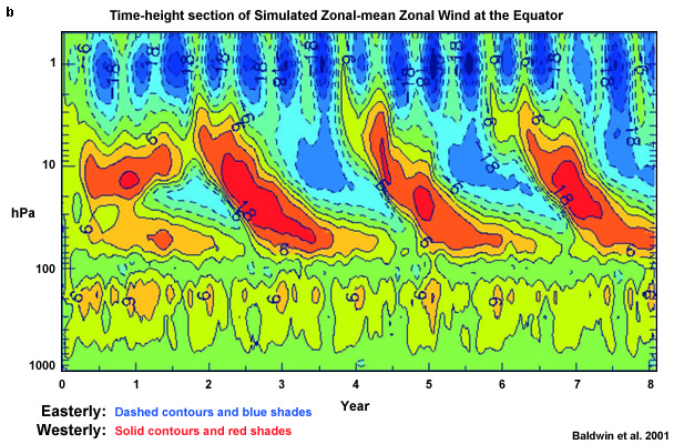
Defining characteristics of the QBO are:
- The period of the oscillation is 20 to 36 months with a mean of around 28 months.
- The oscillation is evident in the zonal winds and, to a lesser extent, the temperature.
- Easterlies are generally stronger than westerlies.
- The QBO signature in the zonal wind propagates downwards with time from roughly 10 hPa to 100 hPa or lower.150
- This downwards propagation proceeds at about 1 km per month.
- Westerly winds last longer than easterly winds at higher levels while easterlies last longer at lower levels.
- The westerlies move down faster than the easterlies, especially in the lower stratosphere (steeper blue to red transition compared to red to blue in Fig. 4.54).
- The QBO amplitude decreases with decreasing height; the maximum amplitude (40–50 m s-1) is generally observed near 20 hPa.
- Transition between westerly and easterly zonal wind regimes is often delayed between 30 and 50 hPa (long yellow “tail” on red anomalies in Fig. 4.54).
- Both the QBO period and amplitude exhibit considerable variability.
In the following figures, latitude-time plots of zonally-averaged zonal winds demonstrate the very strong near equatorial QBO signal at 10 hPa (Fig. 4.55a) and a much weaker QBO signal at 100 hPa (Fig. 4.55b).
While the first two diagnostics we considered focused on near-equatorial zonal winds, the QBO is not confined to the tropics (Fig. 4.55): its influence has been traced to quasi-biennial variations in the subtropical highs and subpolar lows.152
The extension of the QBO into the subtropics is also evident in Fig. 4.55, however the very large variations depicted in the zonal wind amplitudes at high latitudes are predominantly a result of the seasonal cycle.
4.2 Sources of Interannual Variability »
4.2.2 The Quasi Biennial Oscillation (QBO) »
4.2.2.3 Impacts of the QBO on other Atmospheric Phenomena
While the QBO has its largest amplitude in the stratosphere, it has been identified as impacting a wide range of atmospheric phenomena in both the troposphere and stratosphere. We have already discussed how the QBO discovery came from the need to resolve a puzzle about why the plume from the Krakatoa volcano tracked westward (implying easterly flow in the stratosphere) while African balloon observations showed westerlies at that height in the atmosphere. More recently, the decay of aerosol loading for more recent volcanic eruptions (El Chichón in 1982 and Mount Pinatubo in 1991) has been shown to depend on the phase of the QBO.153 Also in the stratosphere, major winter warmings preferentially occur during the easterly phase of the QBO.154
The phase and magnitude of QBO have been associated with the frequency of North Atlantic tropical cyclones (Chapter 8, Section 8.6.3.2).125,133 Hurricanes are more frequent when the 30–hPa winds are westerly; in this phase the vertical wind shear in the upper troposphere and lower stratosphere is reduced. The QBO has also been shown to affect the monsoon, although not as strong as local sea surface temperatures and ENSO. In fact, atmospheric variations associated with ENSO are also affected by the QBO.155 This might explain the QBO link back to the monsoon. Interestingly, while Atlantic TC activity increases for the westerly phase of the QBO (positive zonal wind anomalies) in both the North Atlantic125 and western North Pacific,156 TC numbers in the North Indian Ocean are largest for the easterly QBO (negative zonal wind anomalies).
The phase and magnitude of QBO have been associated with the frequency of North Atlantic tropical cyclones (Chapter 8, Section 8.6.3.2).125,133 Hurricanes are more frequent when the 30–hPa winds are westerly; in this phase the vertical wind shear in the upper troposphere and lower stratosphere is reduced. The QBO has also been shown to affect the monsoon, although not as strong as local sea surface temperatures and ENSO. In fact, atmospheric variations associated with ENSO are also affected by the QBO.155 This might explain the QBO link back to the monsoon. Interestingly, while Atlantic TC activity increases for the westerly phase of the QBO (positive zonal wind anomalies) in both the North Atlantic125 and western North Pacific,156 TC numbers in the North Indian Ocean are largest for the easterly QBO (negative zonal wind anomalies).
One explanation for the variations of TC response to QBO in the different basins is that the QBO does not impact the TC directly, but that the zonal wind shear near the tropopause is reduced for the "active TC" QBO phases in each basin. The reduced zonal wind shear aloft increases the deep convection in the region making it more favorable for TC formation.157 Variations in the Sahel rainfall have been used to demonstrate this link between QBO, convection and Atlantic TC activity.158
4.2 Sources of Interannual Variability »
4.2.2 The Quasi Biennial Oscillation (QBO) »
4.2.2.4 The Theory of the QBO
While various theories have been proposed to explain the QBO, the current theory is that equatorially trapped Kelvin waves provide the westerly momentum and Rossby-gravity waves provide easterly momentum and these effects combine to produce the QBO oscillation.159 We have already discussed these waves, so we will just briefly describe how they contribute to the changing phase of the QBO. Schematics are illustrated in Fig. 4.56.
The westerly jet (the narrow bulge at the bottom right of Fig. 4.56a) prevents the Kelvin waves (red) from propagating any higher, but the mixed Rossby-gravity waves can propagate up to the easterly wind maximum (panel a). As the waves keep depositing momentum around this jet, it gets narrower and narrower in the vertical. Eventually the jet gets too thin and becomes unstable. It mixes with the easterlies– and the westerly jet is mixed away altogether (panel b).
Without the westerly jet barrier, the westerly Kelvin waves (red) can now propagate to high levels through the easterly mean flow, depositing westerly momentum aloft (panel c). As more and more westerly momentum is deposited aloft, this layer expands and the easterlies are forced lower in the atmosphere (panel d). In this way, both the westerlies and easterlies associated with the QBO descend through the atmosphere.
Now the easterly jet below has easterlies deposited below and westerlies above. It eventually becomes unstable and is mixed away like the westerly jet before it, leaving only westerlies at this level (panel e). Now that the easterlies are gone, the mixed Rossby-gravity waves (blue) can transport easterly momentum aloft (panel e). This leads to the formation of a zone of easterlies aloft (panel f) and we are now in the opposite phase of the QBO from where we started.
![]() Continue this description and show how the QBO eventually returns to westerlies aloft.
Continue this description and show how the QBO eventually returns to westerlies aloft.
4.3 Sources of Decadal Variability
In addition to the intraseasonal MJO and interannual ENSO, tropical and extratropical interactions are also correlated on the decadal scale. We will focus on three such relationships in this section.
4.3 Sources of Decadal Variability »
4.3.1 The Pacific Decadal Oscillation (PDO)
The Pacific Decadal Oscillation (PDO),160,161 refers to the oscillation of North Pacific ocean and atmospheric anomalies over a 20–30 year period (Fig. 4.57). The PDO is strongly correlated with ENSO; both reach their highest magnitude during the boreal winter.144 Unlike ENSO, the PDO signature in the tropics is secondary to its signal in the North Pacific and North America. The PDO pattern is similar to the interannual PNA (Section 4.2.1.7).
The Pacific Decadal Oscillation (PDO),160,161 refers to the oscillation of North Pacific ocean and atmospheric anomalies over a 20–30 year period (Fig. 4.57). The PDO is strongly correlated with ENSO; both reach their highest magnitude during the boreal winter.144 Unlike ENSO, the PDO signature in the tropics is secondary to its signal in the North Pacific and North America. The PDO pattern is similar to the interannual PNA (Section 4.2.1.7).
Positive PDO values are usually associated with wetter conditions in the Southwestern US, while negative PDO values are suggestive of persistent drought.160,162 The PDO is also highly correlated with major changes in north Pacific fish populations and marine ecosystems.160 Causes of the PDO are not known, which limits its predictability; although some climate simulations have produced oscillations that are similar to the PDO.
4.3 Sources of Decadal Variability »
4.3.2 The Atlantic Multidecadal Oscillation (AMO)
The Atlantic Multidecadal Oscillation (AMO) Index measures changes in surface temperature and vertical shear of the horizontal winds for large areas of the tropical Atlantic over 20–40 year periods. The AMO influences the extra tropics by shifting the subtropical ridges and jet streams. When the tropical north Atlantic is anomalously warm (positive AMO), less rain falls over most of the US and northeastern South America, and more rain falls in southern Alaska, northern Europe, west Africa, and the southeastern US163 (Fig. 4.58). Persistent drought across the midwest US, such as the 1930s Dust Bowl years, was associated with positive AMO.
The AMO has also been associated with multidecadal Atlantic hurricane activity (Chapter 8, Section 8.6.4). More tropical storms become major hurricanes during the AMO warm phase than during the cool phase164(Fig. 4.59).
The AMO has also been associated with multidecadal Atlantic hurricane activity (Chapter 8, Section 8.6.5). More tropical storms become major hurricanes during the AMO warm phase than during the cool phase164(Fig. 4.59).
4.3 Sources of Decadal Variability »
4.3.3 The North Atlantic Oscillation (NAO)
The North Atlantic Oscillation (NAO)165 is a large-scale seesaw between the subtropical high and polar low in the North Atlantic. The positive NAO is marked by stronger pressure difference between the Bermuda/Azores subtropical high and the Icelandic low and stronger easterlies in the tropical Atlantic. During negative NAO, the subtropical high and Iceland low are weaker and the tropical easterlies weaken. The NAO has its strongest impact on the high latitudes. The link between the NAO and tropical forcing remains open to debate. Some studies suggest an indirect link between ENSO and the NAO.166,167
http://www.ldeo.columbia.edu/res/pi/NAO/
National Center for Atmospheric Research (NCAR),
http://www.cgd.ucar.edu/cas/jhurrell/indices.html
NOAA/CPC, http://www.cpc.noaa.gov/data/teledoc/nao.shtml
Focus Areas
Focus Areas »
Focus 1: Intraseasonal Variability, Tropical Weather, and Tropical Cyclones
This textbook provides new information about the MJO and Equatorial waves that is useful for tropical weather analysis and forecasting. Here we provide a summary list of textbook sections and visual resources on these topics.
The MJO influence on tropical weather
Tropical Weather
The MJO influence on global weather patterns, Section 4.1.1.3The MJO influence on global weather patterns, Section 4.1.1.3 including Figs. 4.10a and 4.10b
Monitoring and Forecasting the MJO, Section 4.1.1.4Monitoring and Forecasting the MJO, Section 4.1.1.4 including a list of real-time forecasts onlinelist of real-time forecasts online.
Tropical Cyclones
MJO phases and tropical cyclones over the Gulf of Mexico and western Atlantic, Section 4.1.1.3MJO phases and tropical cyclones over the Gulf of Mexico and western Atlantic, Section 4.1.1.3, including Fig. 4.8
Tropical cyclone activity modulated by the MJO, Section 8.6.2.1Tropical cyclone activity modulated by the MJO, Section 8.6.2.1, Fig. 8.55
Equatorial waves and tropical weather
Observations of equatorial waves
- Kelvin waves, Figs. 4.15, 4.24a.
- Kelvin waves observed by equatorial radar, Chapter 2, Section 2.2.5Chapter 2, Section 2.2.5
- Equatorial Rossby waves, Section 4.1.2.2Section 4.1.2.2, Figs. 4.16, 4.17, and 4.24b
- Mixed Rossby-Gravity waves, Section 4.1.2.3Section 4.1.2.3 including Fig. 4.18
- Monitoring and forecasting equatorial waves, Section 4.1.5.2Monitoring and forecasting equatorial waves, Section 4.1.5.2 including list of real-time diagnostics and forecasts of equatorial waves.list of real-time diagnostics and forecasts of equatorial waves.
Conceptual models of equatorial waves
Kelvin waves, Animation of Fig. 4.19
Equatorial (n=1) Rossby wave, Animation of Fig. 4.20
Mixed Rossby-Gravity wave, Fig. 4.21
Equatorial waves and tropical cyclones
Equatorial wave impact and tropical cyclone activity, Section 4.1.5.1Equatorial wave impact and tropical cyclone activity, Section 4.1.5.1 including Fig. 4.22
NH and SH twin tropical cyclogenesis from equatorial Rossby waves, Chapter 8, Section 8.3.2.2Chapter 8, Section 8.3.2.2 including animation of Sidr and Lee-Ariel in 2007 (Fig. 8.21)
Tropical cyclogenesis from mixed Rossby-Gravity waves, including animation of Tropical Cyclone 05A over the northern Indian Ocean (Fig. 8.22)
Focus Areas »
Operational Focus
MJO Observations and Impact
Forecasting the MJO
Equatorial Waves and Tropical Weather
Monitoring and Forecasting Equatorial Waves
Observing ENSO
ENSO Impacts
Forecasting ENSO
QBO
Summary
Variability of the tropical atmosphere and oceans impacts the global climate on a range of space and time scales. Understanding the teleconnections within the tropics, such as changes in the Walker circulation due to ENSO, and outside of the tropics, such as changes to storms in the midlatitudes due to ENSO, provides insights into the global climate system. Coherent patterns of tropical variability can be seen locally on diurnal scales, and on increasing space and time scales. Dominant sources of intraseasonal variability include equatorial waves (Kelvin, Rossby, and Mixed Rossby-gravity waves) in atmosphere and ocean, as well as the Madden Julian Oscillation (MJO). The El Niño Southern Oscillation (ENSO) phenomenon is a well recognized driver of interannual variability that is centered in the tropics, but has global impacts. It is perhaps surprising that a Quasi-biennial Oscillation (QBO) in the stratospheric winds also affects the tropical weather and climate. For example, the QBO has been shown to impact tropical cyclone activity in both the North Atlantic and western North Pacific. Finally, decadal variability due to the PDO and AMO produces very long time changes to the tropical climate that may modify patterns of shorter time variations. However, the MJO, ENSO, QBO and other intraseasonal and interannual sources of variability may also feedback and modify longer term signals. Understanding the complicated interactions among these sources of variability will help us to improve forecasts of tropical weather and climate, and will also provide insights into weather and climate variability outside the tropics.
Appendix A: Solving for the Equatorial Wave Form Solutions
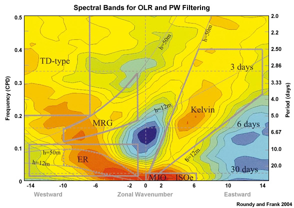
In these appendices we build the fundamental materials to derive the complete waveform solutions for the large-scale equatorial waves discussed in Chapter 5. The shallow water equations (SWE) will be used to derive the wave solutions. To clarify the constraints on the wave solutions, the shallow water equations (SWE) are first derived from the complete (dry) Navier–Stokes equations. Next, we solve for the potential vorticity equation corresponding to the SWE (Appendix A1.5).
In these appendices we build the fundamental materials to derive the complete waveform solutions for the large-scale equatorial waves discussed in Chapter 5. The shallow water equations (SWE) will be used to derive the wave solutions. To clarify the constraints on the wave solutions, the shallow water equations (SWE) are first derived from the complete (dry) Navier–Stokes equations. Next, we solve for the potential vorticity equation corresponding to the SWE (Appendix A1.5).
A derivation of a single equation from the SWE follows. The perturbation method is applied to derive wave form solutions from this equation. This approach leads us to the mathematical solutions for each wave type and to the dispersion relations that give insights into wave and energy propagation for each wave (Appendix B).
A derivation of a single equation from the SWE follows. The perturbation method is applied to derive wave form solutions from this equation. This approach leads us to the mathematical solutions for each wave type and to the dispersion relations that give insights into wave and energy propagation for each wave (Appendix B).
The dispersion relations derived in Appendix B are related back to the frequency‑dispersion diagram pictured above. Finally, the three-dimensional structures of these waves are presented. The appendices draw on ideas described by Adrian Gill,51 Matthew Wheeler,62 and I.N. James.168
The dispersion relations derived in Appendix B are related back to the frequency‑dispersion diagram pictured above. Finally, the three-dimensional structures of these waves are presented. The appendices draw on ideas described by Adrian Gill,51 Matthew Wheeler,62 and I.N. James.168
Appendix A: Solving for the Equatorial Wave Form Solutions »
A1 Derivation of the Shallow Water Equations
Our goal is to find mathematical solutions for each of the large-scale equatorial wave types discussed in this chapter. To keep the derivations as straightforward as possible, we follow the approach pioneered by Matsuno (1966) and employ a simplified form of the Navier Stokes equations known as the Shallow Water Equations (often referred to here as the SWE) to derive the waveform solutions.
First, we will derive the SWE, including the derivation of the relevant form of the potential vorticity equation. In Appendix C, we will use wave solutions from the SWE and a vertical structure function to derive the complete three–dimensional wave structures.
First, we will derive the SWE, including the derivation of the relevant form of the potential vorticity equation. In Appendix C, we will use wave solutions from the SWE and a vertical structure function to derive the complete three–dimensional wave structures.
Appendix A: Solving for the Equatorial Wave Form Solutions »
A1 Derivation of the Shallow Water Equations »
A1.1 Assumptions Implicit in the Shallow Water Equations (SWE) Derivation
Three key assumptions underlie the derivation of the shallow water equations from the dry, adiabatic primitive equation set (i.e. the Navier Stokes equations and the Continuity Equation). The first assumption is that the atmosphere (or ocean, or atmosphere-ocean interface) can be approximated by two distinct layers, each of which is horizontally and vertically homogeneous at rest. While this assumption can become problematic when considering a continuously stratified atmosphere, it can be useful when considering the external (or even the first internal) modes of the atmosphere. The second assumption is that neither the pressure nor density in the upper layer varies in the horizontal. Finally, the third assumption is that the hydrostatic approximation holds.
Taken together, these last two assumptions constrain the pressure gradient force not to vary in the vertical. One can see this for the upper layer by taking the horizontal gradient of the hydrostatic relation
 ,
,since pressure is constrained to have no horizontal variation. Pressure must have horizontal variations in the lower layer, or balanced flows could not be maintained – but even in the lower layer, there is no variation of pressure in the vertical. Considering the horizontal gradient of the hydrostatic relation and remembering that the density in this layer is assumed constant, we see that
The shallow water equations become more straightforward when the pressure is replaced by the vertical depth of the lower layer. For a balanced flow, the winds and pressure must both vary spatially. If the pressure varies, through the hydrostatic approximation, the depth of the fluid must also vary, viz
 .
.Since both density and gravity are constant and (as demonstrated above) pressure does not vary in the vertical, we have shown that horizontal gradients in pressure are equivalent to horizontal gradients in the depth, h, of the fluid. Stir your coffee in a circular motion and look at the surface of the coffee – it will dip down in the center and rise up at the sides. This is an everyday example of the horizontal variation of the depth of a fluid in response to its motion.
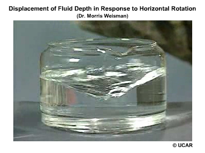
It follows from the pressure gradient being independent of height that wind perturbations in the lower layer will also be height-independent. As a result, there is no vertical advection of the winds.
Appendix A: Solving for the Equatorial Wave Form Solutions »
A1 Derivation of the Shallow Water Equations »
A1.2 Derivation of the Shallow Water Equations in a Rotating Reference Frame
Combining all of the assumptions and the results derived in consequence, the horizontal wind components of the Navier Stokes Equationsi reduce to
where (u, v) is the horizontal wind vector, f is the Coriolis parameter, ρU and ρL are the densities in the upper and lower fluid layersj respectively. The fluid depth, h(x, y, t), has been partitioned into h = H + η, where H is a constant and η(x, y, t). This becomes important later when the equations are linearized to solve for the equatorial waves.
Defining the effective gravity, g′, as  , the momentum equations for the shallow water approximation reduce to

The continuity equation is manipulated to derive the final equation in the shallow water equationk set. Integrating the continuity equation from the ground (where the vertical motion, w, must be zero) to h, the top of the lower fluid, gives
 ,
,since pressure, and therefore (u, v), does not vary in the vertical. Returning to the vertical integration of the continuity equation gives
 ,
,where w(z=h) is the movement of the fluid interface (i.e., the change in time of the lower fluid depth). As a direct consequence of these two results we can write
 .
.which simply says that upward (downward) motion of the lower fluid surface is equal to the depth of the lower fluid times the convergence (divergence) in the lower fluid.
Since  , this last equation can be rewritten as
Finally, recalling our partition for the lower fluid depth in terms of a mean (constant) depth, H, and a spatially and temporally varying perturbation, η(x, y, t), to this depth, we arrive at the final form of the third shallow water equation
 .
.This is simply stating that the movement of the lower fluid interface, h, is equal to the depth of the lower fluid times the convergence in the lower fluid. This means that either more convergence or convergence in a deeper layer will result in a greater change in the fluid depth.
The complete set of the Shallow Water Equations on a rotating Earth are thus
 (1),
(1), (2),
(2), (3).
(3).i We derive the Shallow Water Equations in Cartesian coordinates to keep the mathematics straightforward. They can be readily transformed into spherical coordinates.
j Clearly, for a statically stable system, ρL > ρU and so (ρL – ρU) > 0.
k Recall that we have already used the vertical component of the Navier-Stokes equations through the hydrostatic assumption.
Appendix A: Solving for the Equatorial Wave Form Solutions »
A1 Derivation of the Shallow Water Equations »
A1.3 The Shallow Water Equations on an Equatorial β -Plane
When considering tropical waves, we can further simplify the Coriolis term of the shallow water equations. The following approximation of this equation set to an equatorial β–plane introduces a maximum error of only 14% into the calculations at 30° from the equator (Gill 1982). Thus, we will restrict any analysis based on this form of the equations to the latitude range 30°S 30°N – certainly no hardship for analyses of the tropics!
Making the small angle assumption
 ,
, 
leads to
 ,
, = constant,
where a is the radius of the Earth and is generally taken to be constant (6.37 × 10⁶ m). The Coriolis parameter, f, and its north-south gradient, β, for a β–plane at reference latitude  are thus
 , a constant,
 = 2.3×10⁻¹¹ s-1 m-1 (4).
Using (3) and (4), the Coriolis parameter on a β–plane is
 (5),
(5),where y is the north-south displacement (in meters) away from the reference latitude .
For the special case of a β–plane centered on the equator
 (5)′.
(5)′.Using expression (5)′ in Equations (1) – (3) gives the shallow water equations on an equatorial β–plane
 (1)′,
(1)′, (2)′,
(2)′, (3)′.
(3)′.Appendix A: Solving for the Equatorial Wave Form Solutions »
A1 Derivation of the Shallow Water Equations »
A1.4 Linearizing the Shallow Water Equations on an Equatorial β -Plane
One more simplification – linearization about a quiescent background state – is possible to reduce these equations to only the terms necessary to illuminate the key processes in Rossby, inertia-gravity, mixed Rossby-gravity and Kelvin waves.
First, partition each of the wind components and height field in Equations (1)′ – (3)′ into a mean (background flow) component and a component due to the wave; i.e.


where the variables subscript “TOTAL” are the same variables as in Equations (1)′ – (3)′. The quantities U, V and N are due to the background flow, H is the constant background fluid depth introduced above and  ,
,  and
and  are now the perturbation variables due to the wave. We will explore how to apply this perturbation technique to express the SWE for the waves in Appendix B.
where the variables subscript “TOTAL” are the same variables as in Equations (1)′ – (3)′. The quantities U, V and N are due to the background flow, H is the constant background fluid depth introduced above and , and are now the perturbation variables due to the wave. We will explore how to apply this perturbation technique to express the SWE for the waves in Appendix B.
For a linearization to be valid, the perturbations due to the waves (, and ) must be small. In the midlatitudes this generally corresponds to the ageostrophic component of the motion or something similar.
Assuming U=0, V=0 and N=0 equates to a background state with no motion – and hence no balancing pressure gradient.
Linearizing the shallow water equations on an equatorial β–plane about this state of rest results in the following equations
 (6),
(6), (7),
(7), (8).
(8).Appendix A: Solving for the Equatorial Wave Form Solutions »
A1 Derivation of the Shallow Water Equations »
A1.5 Potential Vorticity Equation for Equatorial β-Plane Shallow Water Equations
Potential vorticity (PV) is a quantity that combines measures of rotation and mass distribution. As a result, it has proven to be a useful property to track balanced flow structures. Hence we will want to incorporate PV into our discussion of waves. Since Equations (6) – (8) incorporate all of the information about the mass and velocity fields of the shallow water system, we can use these to derive the relevant PV equation.
Potential vorticity (PV) is a quantity that combines measures of rotation and mass distribution. As a result, it has proven to be a useful property to track balanced flow structures. Hence we will want to incorporate PV into our discussion of waves. Since Equations (6) – (8) incorporate all of the information about the mass and velocity fields of the shallow water system, we can use these to derive the relevant PV equation.
Taking  and rearranging gives
 .
.Rearranging (8) and substituting into this equation gives
 (9),
(9),where  , the relative vorticity.
Finally, in this linearized system  since
since  ; recognizing that
  (recall that h = (
 ) and using the previous results and log laws, we can rewrite Equation (9) as
 (10),
(10),where q is the barotropic, divergent potential vorticity, defined as
 (11).
(11).Because of our formulation of this linearized system, q is a perturbation quantity and is a measure of the PV of the wave. Equation (10) is the classical formulation for the barotropic, divergent PV equation; it is a statement that q is conserved following the flow. An alternative interpretation is that the temporal evolution of q at a fixed location is governed by the advection of q by the mean flow.
For our purposes, it is more straightforward to expand out the terms in (10). Writing (10) as
 ,
,then taking each of the terms on the right hand side in turn, we see that:
 (i)
(i) (ii),
(ii),Combining terms (i) and (ii) into Equation (10) gives
 ,
,i.e.,
 (12).
(12).Equation (12) is the version of Equation (10) appropriate for the linearized shallow water equations with no background flow. Equations (6) – (8), in combination with Equation (12), form the jumping off point for our derivations of the theoretical solutions to each of the equatorial wave types.
Equation (12) is the version of Equation (10) appropriate for the linearized shallow water equations with no background flow. Equations (6) – (8), in combination with Equation (12), form the jumping off point for our derivations of the theoretical solutions to each of the equatorial wave types.
Appendix B: Derivation of Generalized Dispersion Relation for Waves in the SWE
To explore wave solutions relevant to the Shallow Water Equation set (6) – (8) and (12), we must solve for a consistent set of wave structures in each of the dependent variables (u, v, and h). The most straightforward method is to reduce this equation set to a single equation for one variable and then to substitute back through the equation set to derive consistent wave solutions for the remaining variables.
We will begin from the shallow water equations for an equatorial β–plane linearized about a state of no motion,
 (6),
(6), (7),
(7), (8).
(8).Since we want wave solutions, we will assume solutions for u, v, and h that specify a wave in (x, t) and have an undetermined functional form in y:
 (14a),
 (14b),
and
 (14c),
 where U, V and are the a mplitudes of each variable due to the wave (e.g., U is the largest magnitude of the zonal component of the velocity) and these amplitudes vary in the y-direction (i.e., in the north-south); k is the zonal wavenumber, ω is the wave frequency and
  . As a direct consequence of assuming this form for the variables in the shallow water equations, the following are true
 and
and  (14)′.
Substituting (14a)-(14c) and (14)′ into equations (6)-(8) leads to
 (6)′,
(6)′, (7)′,
(7)′,and
 (8)′.
(8)′.Solving (6)′ for U, then substituting this result into (7)′ and (8)′ gives two coupled equations in V and HW
 (7)′′,
 (8)′′.
Substituting (8)′′ into (7)′′ to eliminate HW and rearranging gives a second order ordinary differential equation in V
 (15).
(15).The solution to Equation (15) gives the functional form of V in the meridional direction. This will complete the specification of the structure of the perturbation meridional velocity component field associated with the wave since the zonal and temporal variations of V have already been specified above. Once this is known, solutions for the structures of the zonal component and the height field can also be obtained.
Consider two asymptotic solutions to Equation (15) to gain insights into the wave types possible in the solution. We will explore these simplified forms of the dispersion relation for this system before returning to the solution for V(y).
Nondivergent limit for Equation (15): 
 (15)′.
 Equation (15)′ will have solutions of the form
 , giving
  (16).
(16).Substituting (16) into (15)′ and rearranging gives
 (17).
(17).Equation (17) is simply the Rossby wave dispersion relation for a quiescent background flow – it is the same dispersion relation as you’ve derived for midlatitude flow. This confirms that equatorial Rossby waves are also potential vorticity conserving waves.
Non-rotating limit for Equation (15): 
 (15)′′,
and using assumptions (16) this becomes
 ,
,or
 (18).
(18).Equation (18) is the dispersion relation for a pair of two-dimensional external gravity waves, one propagating eastwards and one propagating westwards.
So we see that the shallow water equations set supports gravity waves (buoyancy restoring force, so divergent and, in this limit, irrotational) and Rossby waves (PV restoring force, nondivergent).
Back to the general form of the equation governing the meridional structure of these waves
 (15).
(15).We require solutions for Equation (15) such that
 as
as  (19).
(19).Boundary condition (19) constrains the wave solution of (15) to decay away from the equator, ensuring that the wave is bounded and does not extend outside the bounds acceptable for the equatorial β–plane approximation.
Matsuno (1966) showed that solutions to Equation (15) only satisfy boundary conditions (19) if
 , n = 0, 1, 2, 3,... (20),
which ensures that a finite integer number of waves are present in the meridional direction.
Since Equation (20) gives the relationship between the frequency and wavenumber for all possible wave solutions in this system, it is known as the dispersion relation. We will return to this important equation repeatedly.
Multiplying the general form of the dispersion relation (Equation (20)) through by  and rearranging
 (20)′,
showing that this dispersion relation is cubic. Thus, we expect (at most) three unique solutions from Equation (20). However, the special case of Kelvin waves is not captured within this dispersion relation, so that will provide another solution to the shallow water equations wave set.
Appendix C: Equatorial Wave Motion and Structure
We have shown that both gravity and vorticity (Rossby) waves exist in the shallow water wave equations we are using to explore equatorial waves. For those wave scales, the Earth’s rotation will be important, giving inertia-gravity wave solutions (rather than pure gravity waves).
Next, we will explore the structure and motion of these wave types (contained in Equation (20), the dispersion relation we derived in Appendix B), as well as equatorial Kelvin waves.
Next, we will explore the structure and motion of these wave types (contained in Equation (20), the dispersion relation we derived in Appendix B), as well as equatorial Kelvin waves.
In studying each wave, we begin from the general form of the dispersion relation that relates frequency and wavenumber for all possible wave solutions in this system. We can rearrange Equation (20) into the following form:
 , n = 0, 1, 2, 3,... (21).
By making the appropriate assumptions on Equation (21) to isolate each wave type, we will derive the dispersion relation for that wave type and the corresponding structure.
Appendix C: Equatorial Wave Motion and Structure »
C1 Finding the Structural Form of Equatorially Trapped Waves
To find the structural form for Rossby, inertia-gravity, or mixed Rossby-gravity waves, we have to return to Equation (15) from Appendix B, the general form of the equation governing the meridional wave structure:l
 (15).
(15).Using Equation (20), the dispersion relation, Equation (15) gives
 , n = 0, 1, 2, 3,... (22),
which is a form of the Schrödinger Equation for an oscillator. Since we know the Schrödinger Equation (and other people have already solved it for us), we also know that it has solutions of the form
 (23),
(23),where Hn is a Hermite polynomial of order n.169
Following Matsuno (1966),13 we normalize the equations by making the substitution
 (24).
(24).Recall that the Rossby deformation length is
and so
 .
.Equation (25) can now be simplified to
 (23)′.
The formula to determine any Hermite polynomial directly is
 (25)
(25)Using Equation (27) we see that the first two Hermite polynomials are H0(Y)=1 and H1(Y)=2Y. An alternative way to find the Hermite polynomials (without having to use derivatives) is to use H0 and H1 and the following recurrence relation
 (25)′
(25)′Using either Equation (25) or (25)′, we can deduce all Hermite polynomials of higher order: for example, H2= 4Y2– 2.169 Hence, substituting for Y from Equation (24), we have
 for n=0,
 for n<=1,
 for n=2.
See that the order, n, of the Hermite polynomial corresponds to the number of nodes (i.e., the number of zeroes) associated with that polynomial. This means that we can count the number of times the meridional velocity component goes to zero in the north-south direction to find the value of n from observations.
The solutions for V(y) are trapped against the equator since we are on an equatorial β‑plane and (from Equation (15))
 .
.Method of solution for wave structure
To solve for the zonal momentum and mass field to describe the complete structural form for each wave, we can substitute into the shallow water equations (6) – (8):
To solve for the zonal momentum and mass field to describe the complete structural form for each wave, we can substitute into the shallow water equations (6) – (8):
- the appropriate form of Equation (25)′ (such as the examples for n=0, n=1, and n=2 given above)
- the relevant dispersion relation.
We will complete these descriptions of the specific wave structures as we find the corresponding dispersion relations in the following sections.
l Since Kelvin waves have no meridional motion across the equator, we will solve for their structure separately.
Appendix C: Equatorial Wave Motion and Structure »
C2 Equatorial Rossby Waves
From studies of midlatitude weather, we know that Rossby waves are also called planetary waves. Therefore, we expect Rossby waves to have low frequencies (to evolve slowly, on synoptic time scales).
Making the assumption of low frequency (small ω) in Equation (21) allows us to ignore the term  as it becomes much smaller than the remaining terms. As a result, we can rearrange Equation (20) to derive an approximation for the variation of Rossby wave frequency in terms of the remaining variables:
 (26).
(26).The phase speed, c, is the ratio of the frequency to wavenumber of the wave:
 (27),
(27),so we see that Equation (23) corresponds to only westward propagating waves since the denominator is positive definite:
 (26)′.
We can infer the sign of the phase speed (and so the direction of wave propagation) by a simple rule: if the frequency, ω, and wavenumber, k, have the same sign, the wave propagates eastward; if they are of the opposite sign, the wave propagates westward (as here).
The spatial structure of the wave can be derived assigning an appropriate value for n in Equations (26) and (23)′ and solving for the meridional wind component, v. Substituting this solution back into the shallow water equations will give the form for both the zonal wind, u, and the height perturbation.
Appendix C: Equatorial Wave Motion and Structure »
C3 Inertia-Gravity (IG) Waves
For high frequency (large ω) waves, the term –kβ/ω in Equation (21) becomes much smaller than the remaining terms. As a result, we can rearrange Equation (21) to derive an approximation for the variation of Rossby wave frequency in terms of the remaining variables:
For high frequency (large ω) waves, the term –kβ/ω in Equation (21) becomes much smaller than the remaining terms. As a result, we can rearrange Equation (21) to derive an approximation for the variation of Rossby wave frequency in terms of the remaining variables:
 (28).
(28).Using the rule for propagation direction we deduced for Rossby waves, we see that the positive root of Equation (24) corresponds to a eastward propagating inertia-gravity waves (since ω and k have the same sign) and the negative root corresponds to westward propagating inertia-gravity waves (since ω and k have opposite signs).
For large k (small wavelength) and small n, the dispersion of these waves approaches
which is the dispersion relation of pure gravity waves.
The spatial structure of the wave in each propagation direction can be derived by assigning an appropriate value for n in Equations (28) and (23)′ and solving for the meridional wind component, v. Substituting this solution back into the shallow water equations will give the form for both the zonal wind, u, and the height perturbation.
Appendix C: Equatorial Wave Motion and Structure »
C4 Mixed Rossby-Gravity (MRG) Waves
For the special case of MRG waves, we can derive the dispersion relation by setting n=0 in Equation (21):
 .
.In deriving Equation (15) we implicitly assumed that

or else one of the terms must go to infinity (since the coefficient of V is negative). This means that there is no westward propagating gravity wave for n=0. As a result, the allowed roots of this cubic equation (that decay away from the equator) are given by
 (29).
(29).The positive root
 (30)
(30)corresponds to an eastward moving inertia-gravity wave.
The negative root of Equation (25) corresponds to a westward moving wave that resembles an inertia–gravity wave for long zonal scale (k →0) and a Rossby wave for zonal scales characteristic of synoptic-scale disturbances. As a result, this westward moving n=0 wave is known as the mixed Rossby-gravity (or MRG) wave and has a dispersion relation given by
 (31).
(31).To derive the spatial structure of the westward propagating mixed Rossby-gravity wave we assume n=0 in Equations (21) and (23)′ and solve for the meridional wind component. Substituting this solution for v back into the shallow water equations gives the solutions for both the zonal wind, u, and the height perturbation.
Appendix C: Equatorial Wave Motion and Structure »
C5 Equatorially-Trapped Kelvin Waves
Kelvin waves resemble very long equatorially trapped gravity waves. These waves have no meridional motion across the equator. Since our derivation of the other equatorial wave types began with the equation for meridional component of motion (Equation (15) at the equator, to derive the dispersion relation for Kelvin waves we need to return to the shallow water equations (6) – (8):
Kelvin waves resemble very long equatorially trapped gravity waves. These waves have no meridional motion across the equator. Since our derivation of the other equatorial wave types began with the equation for meridional component of motion (Equation (15)) at the equator, to derive the dispersion relation for Kelvin waves we need to return to the shallow water equations (6) – (8):
 (6),
(6), (7),
(7), (8).
(8).Setting v=0, these equations reduce to
 (6)′,
(6)′, (7)′,
(7)′, (8)′.
(8)′.Following the procedure used in Appendix B, we once again assume wave form solutions for the variables u, and η
Following the procedure used in Appendix B, we once again assume wave form solutions for the variables u, and η
and as before, this results in the time and meridional derivatives reducing to
 and
and  (14)′.
From Equation (8)′
 (8)′′.
Substituting this expression for u into Equation (6)′ and rearranging gives the following dispersion relation for equatorially-trapped Kelvin waves
 (32).
(32).The negative root is not retained since it does not decay away from the equator. It is clear that Equation (28) is the dispersion relation for an eastward propagating gravity wave with no meridional motion at the equator.
Returning to Equation (21), our generalized dispersion relation, and setting n=−1 we can recover Equation (28). As a result, Kelvin waves are often labeled as n=−1 waves on dispersion diagrams.
Returning to Equation (21), our generalized dispersion relation, and setting n=−1 we can recover Equation (28). As a result, Kelvin waves are often labeled as n=−1 waves on dispersion diagrams.
Using Equation (28) in the wave form Equations (14)’ and solving for the y-dependence (latitudinal variation) of the amplitudes, we see that the amplitude of the zonal motion varies as
 (33).
(33).Remembering that there is no north-south motion in an equatorially trapped Kelvin wave, we can use Equation (29) in (8)′′ to solve for the perturbation height (pressure) field, η.
Appendix C: Equatorial Wave Motion and Structure »
C6 Summary Dispersion Diagram for Equatorially-Trapped Waves
At the beginning of Appendix A we included one form of a dispersion diagram for the equatorially trapped waves. This diagram summarizes the relative (k, ω) space occupied by each wave type. In other words, it tells us what kind of wavelengths (2π/k) and frequencies we should expect for one wave type compared to another.
At the beginning of Appendix A we included one form of a dispersion diagram for the equatorially trapped waves. This diagram summarizes the relative (k, ω) space occupied by each wave type. In other words, it tells us what kind of wavelengths (2π/k) and frequencies we should expect for one wave type compared to another.
Now that we have a better idea of the wavenumbers and frequencies to expect for each wave type, we can explore more detailed versions of Figure 4A.1 in the cited references.
Questions for Review
- Describe the basic structure of the MJO.
- Describe the role of the MJO in atmospheric and oceanic variability in the tropics.
- Describe one candidate theory for a mechanism of formation of the MJO.
- Describe an equatorial Rossby wave. Be sure to include its length and time scales, pattern of highs and lows, and phase speed.
- What is the restoring mechanism for an equatorial Kelvin wave?
- How could you decide whether a wave packet will continue to have the same spatial pattern?
- How would you identify a mixed Rossby gravity (MRG) wave from a satellite loop?
- Would you expect the MRG wave you identified from the satellite data to move with the theoretical wave speed? Why/why not?
- Describe the Walker Circulation. How does the circulation vary between warm and cool phases of the El Niño Southern Oscillation?
- How are El Niño and the Southern Oscillation related?
- Explain how the El Niño Southern Oscillation affects weather in Australia, Indonesia, and adjacent oceans during winter and summer.
- Describe the typical distribution of surface pressure, sea surface temperature, and surface anomalies across the equatorial Pacific during La Niña.
- How does El Niño affect the synoptic pattern across North America and the North Pacific during boreal winter?
- Several theories have been presented for ENSO; describe at least three of them.
- Describe the strengths and weaknesses of current ENSO forecast models.
- Describe the QBO: at what pressure levels is it most evident? What is its period? What atmospheric constituent can we use to trace the passage of the QBO?
- Give an example of an impact of the QBO on tropical weather or climate.
- Describe the climate patterns that tend to exist across the tropical and north Pacific during the warm phase and cool phase of the Pacific Decadal Oscillation.
- Describe at least one impact of decadal fluctuations on interannual variability.
- Compare and contrast the cool and warm phase of the Atlantic Multidecadal Oscillation in terms of their impact on Atlantic hurricane activity, rainfall in North America, and rainfall in West Africa.
- Describe the characteristics of the NAO and its possible impacts in the tropics.
- Which equatorial waves are theorized to be responsible for some cases of tropical cyclogenesis?
QUIZ
You may also take a quiz and email your results to your instructor.
Biographies
Sir Gilbert Walker
Sir Gilbert Walker used training in applied mathematics to discover some of the planet's most important climate cycles. Born in England in 1868, he was a distinguished student. He graduated from the University of Cambridge with a first-class degree in mathematics in 1890 after achieving the coveted status of senior wrangler, or the top score in the third-year mathematical exams, the year before. While casting around for a suitable position after completing his graduate work, he was hired without any prior meteorological or climatological training to become the Indian Meteorological Department's director. His predecessor had been looking for someone who could bring a more mathematical approach to the job. Indeed, Walker saw that the workings of the atmosphere were too complicated to understand physically with existing science, so he sought to apply statistics and mathematics to work out rough, large-scale relationships between pressure and temperature. Accordingly, he put his staff to work grinding data through calculations as a de facto human computer. With this approach, he uncovered the Walker Circulation, which he noted oscillated in sync with warming waters of the tropical eastern Pacific, forming the basis of our current understanding of the El Niño-Southern Oscillation. In addition, Walker pioneered techniques in statistical forecasting, criteria for statistical significance, and introduced the terms Southern Oscillation, North Atlantic Oscillation, and North Pacific Oscillation. For his work and service he was awarded the Royal Meteorological Society's Symons Gold Medal—its premier award—in 1934.
Dr. Taroh Matsuno
“I got interested in the meteorology in my junior high school year, and more than a half century has passed since I have been involved in this field of meteorology and related studies such as climate change and global environment. I am very happy that I have been able to pursue my career on what I really like.” Taroh Matsuno
In 1957, Matsuno obtained a Physics degree (Geophysics) from the University of Tokyo. He went on to receive both his Masters and doctoral degrees from the University of Tokyo. Professor Matsuno is well known for his research on large-scale dynamics and climate dynamics and stratospheric warming.
Matsuno's contribution to the understanding of tropical waves began with a theoretical paper not immediately recognized fully for the breakthroughs it would engender. In this 1966 paper he performed the first thorough analysis of equatorial waves, documenting the wave types that exist in the tropics and propagate along the "equatorial duct." Those theoretically predicted wave motions were discovered in both the atmosphere and in the oceans. Recent advances in the tracking and prediction of equatorial waves hold great promise for improving tropical forecasting and seasonal prediction, including forecasts of tropical cyclogenesis. Matsuno received recognition for his youthful achievements with an award from the Meteorological Society of Japan in 1970.
Upon receiving his doctorate, Taroh Matsuno became a faculty member at Kyushu University, later moving back to a professorial position at the University of Tokyo, where he served as the Director of the Center for Climate System Research. Professor Matsuno moved to Hokkaido University in 1994. In 1998, he became the Director-General of Frontier Research System for Global Change and also served as the Director of Integrated Modeling Research Program.
Professor Matsuno has been recognized widely, receiving the Meteorological Society of Japan Fujiwara Award in 1992 and the Japan Academy Award in 1997. In 1999, he was awarded the American Meteorlogical Society (AMS) Carl-Gustaf Rossby Medal and he was made an honorary member of the AMS in 2002.
Dr. Roland A. Madden
Roland Madden is well-known for his work in the field of tropical meteorology, long-range predictability, and large-scale traveling waves. Rol Madden grew up in Chicago. He graduated from Loyola University, and then went on to earn his Masters in Geophysical Science at the University of Chicago and his Ph.D. at Colorado State University. He began his career as a weather forecaster in the U.S. Air Force. In 1967, Madden joined the National Center for Atmospheric Research (NCAR) as a research scientist and he remains at NCAR to this day.
Madden's ground breaking work with Paul Julian on intraseasonal oscillations led to the discovery and characterization of the Madden-Julian Oscillation, a 30- to 50-day seesaw of easterly winds and pressure in the equatorial regions of the Indian and western Pacific Oceans. The Madden-Julian Oscillation affects weather from eastern Africa across the Pacific and may play a role in triggering El Niño episodes.
In addition to his pioneering work on intraseasonal tropical variability, Madden teamed with Ramanathan to try to predict when global warming from carbon dioxide and chloroflourocarbons (CFCs) produced by humans would become large enough to be detected. Their 1980 publication predicted that those effects would be evident by 2000. The 2001 report by the Intergovernmental Panel on Climate Change (IPCC) confirmed what Ramanathan and Madden had predicted two decades earlier, the discernment of human impact on Earth's surface temperature.
Madden was honored with the 1983 Editor's award for Monthly Weather Review. In 2002 Madden was presented with the Jule G. Charney Award from the American Meteorological Society (AMS) in recognition of his "pioneering investigations of atmospheric predictability, global waves, and the intraseasonal oscillation."
Dr. Paul R. Julian
Paul Julian received his doctorate from the Pennsylvania State University. Upon completing his degree, Julian moved to Boulder in 1957 to the High Altitude Observatory to work with Walter Orr and Bernard Haurwitz among others. In 1963, Julian joined the rapidly growing synoptic group at NCAR. Years later, he moved to the National Meteorological Center (now the National Centers for Environmental Prediction). After retirement, he designed the WMO's Global Upper Air Network for climate research.
While at NCAR, Julian teamed with Roland Madden to document the 30- to 50-day oscillation that became known as the Madden-Julian Oscillation. Their 1971 and 1972 articles are among the most referenced in tropical meteorology. Paul Julian was made an AMS fellow for his contributions to tropical and operational meteorology.