Table of Contents
- 8.0 Overview
- 8.1 Global Distribution and Monitoring of Tropical Cyclones
- 8.2 Three-Dimensional Structure and Flow Balances
- 8.2.1 Key Structural Features of a Mature Tropical Cyclone
- 8.2.2 Stages of a Typical Tropical Cyclone Lifecycle
- Box 8-3 Record Tropical Cyclone Intensity in the Eastern and Western Hemispheres
- 8.2.3 Mass Balance Solutions and Scaling Considerations
- 8.2.4 Post-landfall Structure
- Box 8-4 Hurricane Mitch (1988): A Devastating Storm in Central America
- 8.3 Tropical Cyclogenesis
- 8.3.1 Necessary Conditions for the Formation of a Tropical Cyclone
- 8.3.2 Dynamic Controls on Genesis in the Monsoon Trough Environment
- Box 8-5 They Lived to Tell the Tale!
- 8.3.3 Mesoscale Influences on Tropical Cyclogenesis
- 8.3.4 Vortex Survival and Evolution
- 8.3.5 Summary of Possible Tropical Cyclogenesis Mechanisms
- 8.4 Intensity
- 8.5 Extratropical Transition (ET)
- 8.6. Climatology of Tropical Cyclones
- 8.6.1 Seasonality of Tropical Cyclone Formation
- Box 8-7 South Atlantic Tropical Cyclone Catarina (2004)
- Box 8-8 Tropical Cyclone Gonu (2007)
- 8.6.2 Intraseasonal Variability
- 8.6.3 Interannual Variability
- 8.6.4 Decadal Cycles and Long Term Climate Influences
- 8.6.5 Seasonal Forecasting of Tropical Cyclone Activity
- Box 8-9 Unusual Tropical Cyclone Seasons around the Globe
- 8.7 Tropical Cyclone Motion
- 8.8 Societal and Environmental Impacts
- Focus Areas
- Summary
- Appendix A: List of Principal Symbols
- Questions for Review
- Brief Biographies
- References
8.0 Overview
This chapter describes tropical cyclones, their history of naming conventions, seasonal and geographic variability and controls, and decadal cycles. The core and balance solutions for regions of the cyclone are examined. Genesis is explored in depth. Intensity scales and satellite interpretation techniques are described. Links between inner core dynamics and changes in intensity are explored. Limits on intensity are considered. Factors that influence motion are described. Extratropical transition is described in terms of structural changes, preceding mechanisms, and impact on high latitudes. The final section describes societal impacts.
Print Version
The print version provides a single printable page with all required content.
Multimedia Version
The multimedia version provides structured page navigation.
Focus Areas
Quiz and Survey
Take a quiz and email your results to your instructor.
After completing this chapter, please submit a User Survey.
8.0 Overview »
Learning objectives
At the end of this chapter, you should understand and be able to:
- Describe tropical cyclone global climatology (where and when they form, where most form, least, or none form)
- Identify distinguishing features of tropical cyclones (eye, eyewall, spiral bands, surface inflow, upper outflow)
- Identify inner core features such as eye-wall vortices
- Describe ingredients needed for formation or genesis (including subtropical genesis)
- Define the stages of a tropical cyclone lifecycle (wave, depression, tropical storm, tropical cyclone, severe tropical cyclone, decay)
- Describe the key storm and environmental factors impacting intensity change
- Using satellite remote sensing, describe how you could detect changes in intensity of tropical cyclones
- Describe the links found between inner core dynamics and changes in cyclone structure and intensity
- Describe the mechanisms that influence tropical cyclone motion from its precursor tropical wave to its landfall in a midlatitude continent
- Describe various mechanisms that lead to extratropical transition
- Describe the hazards of tropical cyclones particularly those at landfall (storm surge, heavy rain and floods, strong winds, tornadoes, ocean waves) and understand the basic mechanisms for each type of hazard
Note that the following sections are highly theoretical; experience in dynamic meteorology is recommended:
- Section 8.2.3
- Box 8-6
- Section 8.7.1
8.1 Global Distribution and Monitoring of Tropical Cyclones
Tropical cyclones have impacted the course of history, confounding the attempts of the Kublai Khan to invade Japan in 12661,2 and changing the course of early European settlement3 in North America. We have also witnessed 20th century tropical cyclones bringing devastation to all of the continents with footholds in the tropics: names such as Tracy (Australia), Bhola (Bangladesh), Mitch and Katrina (the Caribbean, Mexico, Central America and the United States) bring to mind tragedy to millions around the world.
Fig. 8.1 illustrates some key things about the global distribution of tropical cyclones:
- Tropical cyclones do not form very close to the equator and do not ever cross the equator;
- The western North Pacific is the most active tropical cyclone region. It is also the region with the largest number of intense tropical cyclones (orange through red tracks);
- Tropical cyclones in the western North Pacific and the North Atlantic can have tracks that extend to very high latitudes. Storms following these long tracks generally undergo extratropical transition;
- The North Indian Ocean (Bay of Bengal and Arabian Sea) is bounded by land to the north and the eastern North Pacific is bounded by cold water to the north. These environmental features limit the lifetimes of storms in these regions.
- The Bay of Bengal has about five times as many tropical cyclones as the Arabian Sea. The high mountain ranges and low-lying coastal plains and river deltas of the Bay of Bengal combine to make this region extremely vulnerable to tropical cyclones. Indeed, the two most devastating tropical cyclones on record occurred in this region (Box 8-10Box 8-10).
- Southern Hemisphere tropical cyclones are generally weaker than storms in the North Pacific and Atlantic basins;
- The extension of the subtropical jet into tropical latitudes in the Southern Hemisphere acts to constrain the tracks of tropical cyclones. Even so, a few Southern Hemisphere tropical cyclones undergo extratropical transition;
- Although rare, systems resembling tropical cyclones can occur in the South Atlantic Ocean and off the subtropical east coasts of Australia and southern Africa.
Tropical cyclone monitoring occurs in almost every country impacted by these systems. Since tropical cyclones do not observe political boundaries, the WMO has designated official forecasting centers clarify regional forecasting responsibilities. Although the WMO applies a standard definition of tropical cyclone intensity (10-minute mean of the 10-meter wind), many countries have developed their own measures of intensity. Further, regional terms and intensity designations for tropical cyclones have historical roots in each region. These regional variations can confuse our discussions of tropical cyclones around the world. Thus, we will begin our study of tropical cyclones with a typical tropical cyclone case study followed by a review of these rather prosaic regional aspects of tropical cyclone monitoring, including the inadvertent aircraft monitoring described in Box 8-5. This material will provide us with the reference frame for a comprehensive study of tropical cyclones around the globe.
Tropical cyclone monitoring occurs in almost every country impacted by these systems. Since tropical cyclones do not observe political boundaries, the WMO has designated official forecasting centers clarify regional forecasting responsibilities. Although the WMO applies a standard definition of tropical cyclone intensity (10-minute mean of the 10-meter wind), many countries have developed their own measures of intensity. Further, regional terms and intensity designations for tropical cyclones have historical roots in each region. These regional variations can confuse our discussions of tropical cyclones around the world. Thus, we will begin our study of tropical cyclones with a typical tropical cyclone case study followed by a review of these rather prosaic regional aspects of tropical cyclone monitoring, including the inadvertent aircraft monitoring described in Box 8-5. This material will provide us with the reference frame for a comprehensive study of tropical cyclones around the globe.
8.1 Global Distribution and Monitoring of Tropical Cyclones »
Box 8–1 Tropical Cyclone Ingrid, 3-16 March 2005
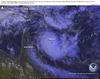
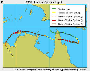
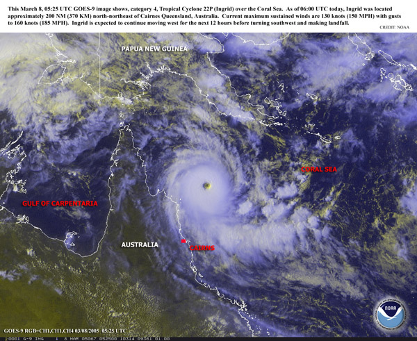
During its 10 days as a tropical cyclone, tropical cyclone Ingrid (2005) remained in close proximity to the northern Australian coast (Fig. 8B1.1) impacting many population centers in the Northern Territory and the states of Queensland and Western Australia as a Cat 4 or 5 tropical cyclone (Australian intensity categories; Box 8-2).
During its 10 days as a tropical cyclone, tropical cyclone Ingrid (2005) remained in close proximity to the northern Australian coast (Fig. 8B1.1) impacting many population centers in the Northern Territory and the states of Queensland and Western Australia as a Cat 4 or 5 tropical cyclone (Australian intensity categories; Box 8-2).
A tropical low developed in the eastern Arafura Sea in an environment with both low vertical shear and anomalously warm SST on 3 March 2005 and was named Tropical Cyclone Ingrid on 6 March. Tropical Cyclone Ingrid developed to a Category (Cat) 5 system by 8 March and around 0600 CST on 10 March Ingrid made landfall on Cape York as a Cat 4 tropical cyclone. Ingrid weakened during its passage over the peninsula, emerging into the Gulf of Carpentaria late on 10 March as a Cat 1 tropical cyclone.
Ingrid skirted the "Top End" of the Northern Territory on 12 and 13 March impacting many coastal communities. Ingrid regained Cat 5 intensity at 2330 UTC on 14 March. Ingrid weakened rapidly after making landfall near Kalumburu in Western Australia, but continued to be an intense rain event (in Wyndham 272 mm of rainfall was recorded in 48 hours).
"Land's eye-views" of Tropical Cyclone Ingrid (2005)

A video of Ingrid's passage over Cape Don on the Cobourg Peninsula
A 5-minute animation from Gove radar, 11 March 2005 commencing at 1701 UTC
Gove set a new record daily rainfall for March of 192 mm to 9 AM on 12 March.
8.1 Global Distribution and Monitoring of Tropical Cyclones »
8.1.1 Naming Conventions and Tropical Cyclone Intensity Classifications
Tropical cyclones have impacted the consciousness of the local populations in regions affected such that local designations for these storms pre-date the current naming conventions. The generic name "tropical cyclones" may be used anywhere in the world for tropical storms with peak wind speeds (1-minute mean, 10-minute mean or gust wind speed are used in different regions) exceeding 17 m s-1. In 18484 the word "cyclone" was first used to refer to rotating storms. This term was inspired by the Greek word Κυκλωζ which means "coiled like a snake." In the western North Pacific, the strongest of these storms (peak wind speeds exceeding 33 m s-1) are called "typhoons."4 The derivation of the term typhoon is still debated and may derive from Greek, Chinese, or Arabic but came into common use first in Japan4 In the Caribbean—and, more recently, in the eastern Pacific—the strongest of these storms are also referred to as "hurricanes" after the Carib god of evil, Hurican. A complete summary of the intensity range naming conventions for each basin is given in Box 8-2.
Tropical cyclones have impacted the consciousness of the local populations in regions affected such that local designations for these storms pre-date the current naming conventions. The generic name "tropical cyclones" may be used anywhere in the world for tropical storms with peak wind speeds (1-minute mean, 10-minute mean or gust wind speed are used in different regions) exceeding 17 m s-1. In 18484 the word "cyclone" was first used to refer to rotating storms. This term was inspired by the Greek word Κυκλωζ which means "coiled like a snake." In the western North Pacific, the strongest of these storms (peak wind speeds exceeding 33 m s-1) are called "typhoons."4 The derivation of the term typhoon is still debated and may derive from Greek, Chinese, or Arabic but came into common use first in Japan4 In the Caribbean—and, more recently, in the eastern Pacific—the strongest of these storms are also referred to as "hurricanes" after the Carib god of evil, Hurican. A complete summary of the intensity range naming conventions for each basin is given in Box 8-2.
While the variety of appellations for tropical cyclones is a little cumbersome, it reflects the local culture and history relating to these important weather systems. However, there is one more wrinkle in the classification of these storms: the averaging time used to measure the peak winds differs around the globe! The World Meteorological Organization (WMO) convention for recording peak wind speeds is to record the 10-minute average surface wind speed; however, the United States only applies a 1 minute average to the instruments' surface wind speed measurements. Thus, it is typical for a western North Pacific storm to be assigned two very different intensities depending on whether recorded by one of the national meteorological agencies of the region (Fig. 8.3) or the US Joint Typhoon Warning Center (JTWC) in Pearl Harbor.
Accurate observational records are not always available after the passage of a tropical cyclone. The instruments may have been blown or washed away – or the instruments may not be located in the path of the storm. Thus, in the late 1960s Herb Saffir and Robert Simpson5,6 devised a classification convention to relate the observed damage due to a North Atlantic tropical cyclone with the peak surface winds or minimum surface pressure (two measures of the "intensity" of a tropical cyclone) and storm surge in vulnerable coastal locations. The classification system became known as the "Saffir–Simpson Scale" and has become shorthand for describing the destructive power expected from tropical cyclones around the world. The Saffir–Simpson scale was updated by the National Hurricane Center (NHC) in early 2010.a The 2010 update removed both central pressure and storm surge from the Saffir–Simpson scale. In March 2012, the wind speeds for Categories 3-5 hurricanes were modified to resolve rounding issues associated with conversion between units. With the previous range, a Category 4 hurricane at 115kt would be rounded to 130mph; which is Category 3 in mph. With the new range, the categories match across units.
Wind |
Storm surge and wind |
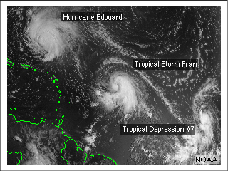
The concept of assigning individual names to tropical cyclones was initiated in the late 19th century by an Australian meteorologist, Clement Wragge.7,8 Wragge used the Greek alphabet and names of politicians whom he did not like. Later, the names came from the military alphabet. In the 1960s the WMO stepped in and developed a consistent, regionally-applicable naming convention for tropical cyclones in each of the affected ocean basins. While the early lists consisted only of women's names, by the 1970s the lists were broadened to include both male and female names and to encompass the languages of all of the affected countries. The names of people are no longer used for storms in the western North Pacific: storm names for this region are drawn from a list of generic words.
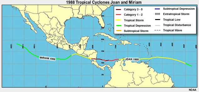
If a tropical cyclone moves from one region to another, it is typically renamed to the next name on the list in the new region. This means that in rare cases, the same storm is assigned two names depending on its track (Fig. 8.2).
WMO, http://www.wmo.int/pages/prog/www/tcp/documents/FactShtTCNames1July05.pdf
NOAA National Hurricane Center, http://www.nhc.noaa.gov/aboutnames.shtml
a Central pressure was used as a proxy for wind speed prior to 1990, since accurate wind speed measurements from aircraft reconnaissance were not routinely available until then. The storm surge scale was shown to be invalid, as the surge is affected by parameters such as storm size and past motion and local bathymetry.
8.1 Global Distribution and Monitoring of Tropical Cyclones »
Box 8–2 Classification of Tropical Cyclone Intensity around the World
Tropical cyclone classification schemes for the different regions are summarized here. Where associated damage is provided it refers to the expected damage in the maximum wind zone. Damage will vary depending upon: (1) distance from the zone of maximum winds; (2) exposure of the location (i.e., sheltered or not); (3) building standards; (4) vegetation type; and (5) resultant flooding and wave action. The effects of storm surge, tide, or wave action are not explicitly included in the classifications.
North Atlantic and Eastern North Pacific: Saffir-Simpson Scale
The Saffir–Simpson scale was initially intended to provide a link between the observed damage and the effects of wind, pressure and storm surge that could lead to such damage. In the first table, the hurricane categories are related to maximum sustained winds (1–minute average and 10 meters above ground) and minimum central pressure. Maximum wind speed is used to determine the category of a hurricane.
Saffir-Simpson Hurricane Category |
Maximum Sustained Wind Speed (VMAX; 1-minute average)b |
Expected Level of Damage |
||
m s-1 |
km h-1 |
mph |
||
1 |
33–42 |
119–153 |
74–95 |
Minimal |
2 |
43–49 |
154–177 |
96–110 |
Moderate |
3 |
50–58 |
178–208 |
111–129 |
Extensive |
4 |
59–69 |
209–251 |
130–156 |
Extreme |
5 |
70+ |
252+ |
157+ |
Catastrophic |
Australian Region: Gust Wind Speed Ranges for Tropical Cyclones
A tropical cyclone scale linking maximum gust (3–5 second, 10 meter) wind speeds to expected damage in the maximum wind zone has been instituted in the Australian Region. As with the Saffir–Simpson scale, the weakest tropical cyclones are designated as Category 1, with the strongest possible tropical cyclones being assigned Category 5.
Categories |
Range of strongest gusts |
Summary Description of Typical Damage Expected |
|
(km h-1) |
(m s-1) |
||
| 1 | < 125 | < 34 | Negligible house damage. Damage to some crops, trees and caravans. |
| 2 | 125 – 170 | 34 – 47 | Minor house damage. Significant damage to trees and caravans. Heavy damage to some crops. Risk of power
failure. |
| 3 | 170 – 225 | 47 – 63 | Some roof and structural damage. Some caravans destroyed. Power failure likely. |
| 4 | 225 – 280 | 63 – 78 | Significant roofing loss and structural damage. Many caravans destroyed and blown away. Dangerous airborne debris. Widespread power failure. |
| 5 | > 280 | > 78 | Extremely dangerous with widespread destruction. |
Western North Pacific and Indian Ocean Tropical Cyclone Intensity
The tropical cyclone intensity scale in these last three basins is based upon the maximum sustained (10–minute average) surface (10 meter) wind speeds. While the wind speed ranges in these basins are consistent, their naming conventions vary.
Range of 10-min mean wind (km h-1) |
Range of 10-min mean wind (m s-1) |
Categories
by Region |
||
Western North Pacific |
North Indian |
South Indian |
||
60 – 119 |
17 – 33 |
Tropical Storm |
Tropical Storm |
Tropical Storm |
120 – 227 |
34 – 63 |
Typhoon |
Severe Cyclonic Storm |
Tropical Cyclone |
> 227 |
>63 |
Super Typhoon |
Severe Tropical Cyclone |
|
Updated Saffir-Simpson Categories 3-5, http://www.nhc.noaa.gov/news/20120301_pis_sshws.php
Updated Saffir-Simpson Hurricane Wind Scale, http://www.nhc.noaa.gov/aboutsshs.shtml
Damage expected for Hurricane categories,
http://www.nhc.noaa.gov/sshws_table.shtml?large
Joint Typhoon Warning Center (US), http://www.usno.navy.mil/JTWC
Australian Bureau of Meteorology, http://www.bom.gov.au
b Use the following conversions for units of wind speed: 1 m s-1 = 3.6 km h-1, 1.94 knots, and 2.237 mph.
8.1 Global Distribution and Monitoring of Tropical Cyclones »
8.1.2 Who is Responsible for Monitoring and Warning on Tropical Cyclones?
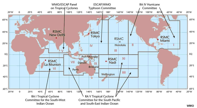
There are six tropical cyclone Regional Specialized Meteorological Centres (RSMCs) together with five Tropical Cyclone Warning Centres (TCWCs) around the world. These centers have been designated as regional warning centers for tropical cyclones (including tropical depressions). Together, these centers cover all regions of the global tropics affected by tropical cyclones. A list of the RSMCs and TCWCs as well as webpage links to these centers is given in Table 8.1. Note that, while the US Navy/Air Force Joint Typhoon Warning Center (JTWC) is not a designated warning center, its forecasts and archive information are also widely used. Other centers that are not designated centers, but make more localized forecasts include the Hong Kong Observatory, The Shanghai Weather Bureau, and the Korean Meteorological Agency.
The RSMCs and TCWCs have responsibility to provide advisories and bulletins with up–to–date first level basic meteorological information on all tropical cyclones to their regions. First level basic meteorological information includes track and intensity observations and forecasts, but may also include a detailed discussion of the underlying reasoning leading to the forecasts and other information that is available to that center (e.g., satellites, computer forecast model outputs). These and the above-mentioned national centers also prepare comprehensive best track archives of tropical cyclones in their warning area.
http://www.wmo.ch/pages/prog/www/tcp/Advisories-RSMCs.html.
Tropical Cyclone Regional Specialized Meteorological Centres (RSMCs) |
|
RSMC Miami-Hurricane Center NOAA/NWS National Hurricane Center (NHC), USA. |
Caribbean Sea, Gulf of Mexico, North Atlantic and eastern North Pacific Oceans http://www.nhc.noaa.gov/index.shtml |
RSMC Tokyo-Typhoon Center Japan Meteorological Agency |
Western North Pacific Ocean and
South China Sea http://www.jma.go.jp/en/typh/ |
RSMC-tropical cyclones New Delhi India Meteorological Department |
Bay of Bengal and the Arabian Sea http://www.imd.gov.in |
RSMC La Réunion-Tropical Cyclone Centre Météo-France |
South-West Indian Ocean http://www.meteo.fr/temps/domtom/ La_Reunion/TGPR/saison/saison_trajGP.html |
RSMC Nadi-Tropical Cyclone Centre Fiji Meteorological Service |
South-West Pacific Ocean http://www.met.gov.fj |
RSMC Honolulu-Hurricane Center NOAA/NWS, USA |
Central North Pacific Ocean http://www.prh.noaa.gov/hnl/cphc/ |
Tropical Cyclone Warning
Centres (TCWCs) with Regional Responsibility |
|
TCWC-Perth Bureau of Meteorology, Australia |
South-East Indian Ocean http://www.bom.gov.au/weather/wa/cyclone/ |
TCWC-Darwin Bureau of Meteorology, Australia |
Arafura Sea and the Gulf of Carpentaria http://www.bom.gov.au/weather/cyclone/ |
TCWC-Brisbane Bureau of Meteorology, Australia |
Coral Sea http://www.bom.gov.au/weather/cyclone/ |
TCWC-Wellington Meteorological Service of New Zealand, Ltd. |
|
TCWC-Jakarta Badan Meteorologi and Geofisika |
Maritime Continent http://www.nhc.noaa.gov/index.shtml |
http://www.wmo.int/pages/prog/www/tcp/index_en.html
US Naval Research Lab (NRL), http://www.nrlmry.navy.mil/tc_pages/tc_home.html
University of Wisconsin, Cooperative Institute for Meteorological Satellite Studies (CIMSS), http://cimss.ssec.wisc.edu/tropic2/
8.2 Three-Dimensional Structure and Flow Balances
A tropical cyclone is a warm-core, non-frontal, low pressure system that develops over the ocean and has a definite organized surface circulation.9
What does this really mean? Let us pause here and examine the the detailed structure of a classic tropical cyclone. First, we examine the fundamental features of the system, and then focus more on the details of the eye of the storm. Next, we consider balanced flow solutions and how they can help us to delineate different regions of the storm. Finally, changes in storm structure associated with landfall are briefly reviewed.
8.2 Three-Dimensional Structure and Flow Balances »
8.2.1 Key Structural Features of a Mature Tropical Cyclone
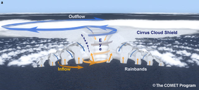
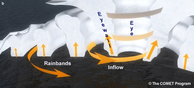
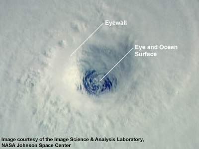
A few structural elements are common to all tropical cyclones. The (i) boundary layer inflow, (ii) eyewall, (iii) cirrus shield, (iv) rainbands, and (v) upper tropospheric outflow (Fig. 8.4) are found in all tropical depressions and tropical storms. As these storms become more intense, a (vi) clear central eye becomes visible from satellite (Fig. 8.5).
Animation of satellite images of TC inflow and outflow,
http://www.comet.ucar.edu/nsflab/web/hurricane/324.htm
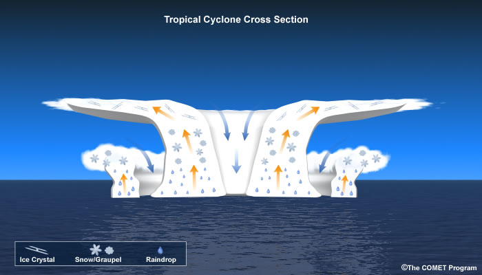
Tropical cyclones are synoptic-scale low pressure systems, so must spin cyclonically. This means that tropical cyclones spin counter-clockwise in the Northern Hemisphere (NH) and clockwise in the Southern Hemisphere (SH), with corresponding variations in their spiral rainband structure. In a tropical cyclone, the wind flows inward cyclonically at lower levels, spiraling upward in the zones of deep convection (the central eyewall or the spiral rainbands), spiraling outward aloft, just below the tropopause (Fig. 8.4). The interactive version of Fig.8.4 illustrates many fundamental aspects of tropical cyclone systems.
The clear region in the center of a mature tropical storm is known as the eye and is relatively calm with light winds and the lowest surface pressure. An organized band of thunderstorms immediately surrounds the calm, storm center. This region is the eyewall and the strongest winds are to be found on the inner flank of this thunderstorm annulus (Fig. 8.5).
The following animation of the evolution of Hurricane Isabel (2003) demonstrates the development of the clear eye as the storm intensifies; eyewall vortices and development of an asymmetric eye, which then resymmetrizes are also evident.
A close-up satellite view of Isabel's eye,
http://tropic.ssec.wisc.edu/storm_archive/2003/storms/isabel/isabel.html (click on the 11th first)
Fly through the storm, http://www.aoml.noaa.gov/hrd/Storm_pages/isabel2003/eye_small.mov
Friction slows the winds near the surface, resulting in convergence in the cyclonic boundary layer flow which spirals into the eyewall forcing dynamically-driven convection (Fig. 8.4b). Under the eyewall, this convergence is enhanced due to the "frontal" zone between the moist inward frictional flow and the dry subsident air flowing outwards from the eye, so air ascending in the eyewall convection comes both from the eye and the outer regions of the storm (interactive Fig. 8.4). For a steady state storm (one that is not changing with time), mass conservation requires subsidence in the eye to compensate for the air rising in the convection. The clear eye results from this subsidence (Fig. 8.6). In weaker storms, the eye may not be evident from visible and infrared satellite images. Thermal (convective) instability may enhance the eyewall convection, contributing to overshooting convection into the stratosphere.
The frictionally-slowed surface wind speed is less than the gradient wind expected from the observed pressure gradient (Section 8.2.3.1). Interestingly, the ratio between these two wind speeds varies with radius: gradient wind balance operates10,11 inside the radius of maximum winds; winds near the eyewall are about 90% of the gradient wind expected there; and winds outside the eyewall are an even lower percentage of the local gradient wind. Observations of the tropical cyclone boundary layer using GPS dropsondes have identified well-defined jet structures in the storm boundary layer.12 The proposed explanation for these jets is that they result from radial import of higher angular momentum air10,11 above the surface.
The frictionally-slowed surface wind speed is less than the gradient wind expected from the observed pressure gradient (Section 8.2.3.1). Interestingly, the ratio between these two wind speeds varies with radius: gradient wind balance operates10,11 inside the radius of maximum winds; winds near the eyewall are about 90% of the gradient wind expected there; and winds outside the eyewall are an even lower percentage of the local gradient wind. Observations of the tropical cyclone boundary layer using GPS dropsondes have identified well-defined jet structures in the storm boundary layer.12 The proposed explanation for these jets is that they result from radial import of higher angular momentum air10,11 above the surface.
Lower to mid-tropospheric convergence above the boundary layer9 can also entrained drier air into the rainbands, contributing to the weaker convection in these bands, compared to the eyewall. The image of the rainbands spiraling out from the eyewall is one of the most recognized satellite signatures today (Fig. 8.5).
In contrast to the conventional view of an isothermal9 tropical cyclone boundary layer, recent observations have shown13 that the storm boundary layer is only isothermal inside the high wind region (about 1.25° radius from the storm center).13,14 These new insights into the hurricane boundary layer structure have consequences for understanding the complete hurricane system.c
Brief description, http://www.aoml.noaa.gov/hrd/nhurr97/GPSNDW.HTM
Detailed technical information, http://www.eol.ucar.edu/rtf/facilities/dropsonde/gpsDropsonde.html
c One example of this is the Carnot engine model for tropical cyclone potential intensity (discussed in Section 8.4): an isothermal boundary layer is assumed as a key aspect of the intensity calculations.
8.2 Three-Dimensional Structure and Flow Balances »
8.2.2 Stages of a Typical Tropical Cyclone Lifecycle
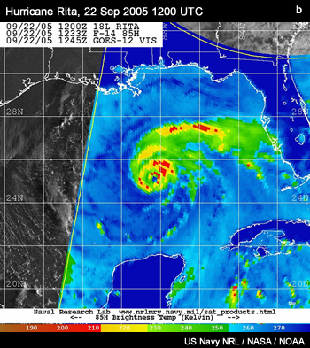
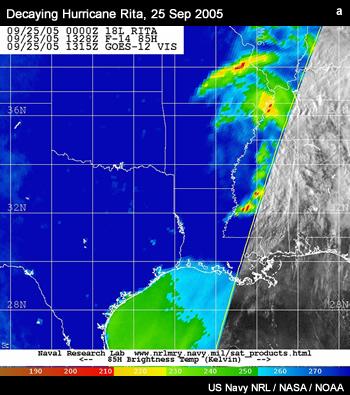
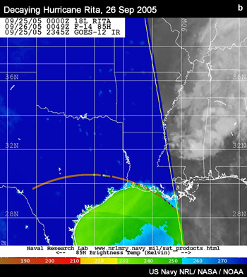
The key stages in the lifecycle of a typical tropical cyclone are incipient disturbance, tropical storm, tropical cyclone (hurricane, typhoon), and possibly severe tropical cyclone (major hurricane, supertyphoon). Having reached its peak intensity at one of these stages (see Box 8-3) for storm intensity classifications, the storm will either decay or undergo extratropical transition. These stages are associated with changes in the storm intensity and structure. In this section, we review the physical stages of the storm lifecycle as illustrated by the stages of Hurricane Rita (Figs. 8.7–8.11).
The key stages in the lifecycle of a typical tropical cyclone are incipient disturbance, tropical storm, tropical cyclone (hurricane, typhoon), and possibly severe tropical cyclone (major hurricane, supertyphoon). Having reached its peak intensity at one of these stages (see Box 8-3) for storm intensity classifications, the storm will either decay or undergo extratropical transition. These stages are associated with changes in the storm intensity and structure. In this section, we review the physical stages of the storm lifecycle as illustrated by the stages of Hurricane Rita (Figs. 8.7–8.11).
8.2 Three-Dimensional Structure and Flow Balances »
8.2.2 Stages of a Typical Tropical Cyclone Lifecycle »
8.2.2.1 Incipient Disturbances
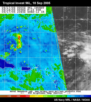
A tropical cyclone will not develop instantaneously: some intermediate, weaker disturbance is needed to provide the "seed" from which a tropical cyclone can develop (Fig. 8.7). In contrast to our expectations for a tropical cyclone, the incipient disturbance can be very asymmetric. A detailed discussion of the sources of disturbances is presented in Section 8.3, so only a few key points are reviewed here.
A tropical cyclone will not develop instantaneously: some intermediate, weaker disturbance is needed to provide the "seed" from which a tropical cyclone can develop (Fig. 8.7). In contrast to our expectations for a tropical cyclone, the incipient disturbance can be very asymmetric. A detailed discussion of the sources of disturbances is presented in Section 8.3, so only a few key points are reviewed here.
A promising incipient disturbance is one that satisfies all of the necessary, but not sufficient, conditions for tropical cyclogenesis (Section 8.3.1); these can be summarized as a low-level cyclonic vorticity maximum in weak vertical wind shear and associated with deep convection. Disturbances meeting these criteria differ in their own formation histories in the different tropical ocean basins:
A promising incipient disturbance is one that satisfies all of the necessary, but not sufficient, conditions for tropical cyclogenesis (Section 8.3.1); these can be summarized as a low-level cyclonic vorticity maximum in weak vertical wind shear and associated with deep convection. Disturbances meeting these criteria differ in their own formation histories in the different tropical ocean basins:
- Western Pacific and Indian Oceans: The monsoon trough is the dominant location for tropical cyclogenesis in the Pacific15 and Indian Oceans, but equatorial Rossby (Fig. 8.21) and mixed Rossby gravity waves (Fig. 8.22) are increasingly being recognized as potential initiators of tropical cyclogenesis in these basins (Fig. 8.30a). Further, merger of a number of smaller (weaker vorticity) mesoscale systems has also been identified as a mechanism for tropical cyclogenesis in the North Pacific16 (Section 8.3.3.3Section 8.3.3.3).
- Eastern Pacific: Tropical storms forming in the eastern North Pacific have been identified with both instabilities in the ITCZ17,18,19 (Section 8.3.2.1Section 8.3.2.1) and with moist easterly waves20 and equatorial waves21 intruding from the Atlantic (Section 8.3.2.1Section 8.3.2.1).
- Atlantic Ocean: The monsoon in the Atlantic basin is mainly confined to West Africa. Easterly waves forming here are influenced by local convection and mesoscale systems that initiate near the Aïr Mountains, Jos Plateau, and Guinea Highlands. As illustrated in Figure 8.24b, they are typically less symmetric than the classic inverted-V satellite signature first reported by Frank22 Another source of Atlantic tropical cyclogenesis is subtropical cyclones (Section 8.3.3.2Section 8.3.3.2); the potential importance of subtropical cyclones to tropical cyclogenesis has yet to be documented in other basins. Subtropical cyclones typically form at the equatorward extreme of a midlatitude frontal zone.23
8.2 Three-Dimensional Structure and Flow Balances »
8.2.2 Stages of a Typical Tropical Cyclone Lifecycle »
8.2.2.2 Tropical Storm

Given a favorable environment, an incipient disturbance may organize into a tropical storm. Maintenance of these favorable environmental conditions for tropical cyclogenesis is ideal for further intensification to the tropical storm stage (Fig. 8.8). The warm ocean waters of the tropics provide the energy source for the tropical cyclone. Evaporation (latent heat flux) and heat transfer (sensible heat flux) from the ocean surface warm and moisten the tropical storm boundary layer. The heat and moisture fluxes and the potential energy comprise the moist static energy of the air (Chapter 5, Section 5.2.3). Conversion of this moist static energy into kinetic energy via convection is the mechanism by which a tropical cyclone intensifies. Later in this chapter we will explore theories for the potential intensity (PI) possible for a storm (Section 8.4.1) based on this mechanism and the reasons why every storm does not achieve its potential intensity (Section 8.4.3).
Given a favorable environment, an incipient disturbance may organize into a tropical storm. Maintenance of these favorable environmental conditions for tropical cyclogenesis is ideal for further intensification to the tropical storm stage (Fig. 8.8). The warm ocean waters of the tropics provide the energy source for the tropical cyclone. Evaporation (latent heat flux) and heat transfer (sensible heat flux) from the ocean surface warm and moisten the tropical storm boundary layer. The heat and moisture fluxes and the potential energy comprise the moist static energy of the air (Chapter 5, Section 5.2.3). Conversion of this moist static energy into kinetic energy via convection is the mechanism by which a tropical cyclone intensifies. Later in this chapter we will explore theories for the potential intensity (PI) possible for a storm (Section 8.4.1) based on this mechanism and the reasons why every storm does not achieve its potential intensity (Section 8.4.3).
Operational centers require a consistent definition — peak surface wind speed — to decide when a system has become a tropical storm, but this is not always the most helpful definition for explaining the storm evolution. Tropical disturbances require external forcing to be sustained. Thus, a physically-based definition of the transition from a tropical disturbance to a tropical storm is that the system has become a tropical storm once it is self-sustaining. This means that, while external forcing might help or hurt the evolution of the tropical storm, it does not need external forcing to remain a coherent system, or even to intensify.
8.2 Three-Dimensional Structure and Flow Balances »
8.2.2 Stages of a Typical Tropical Cyclone Lifecycle »
8.2.2.3 Tropical Cyclone (typhoon, hurricane)
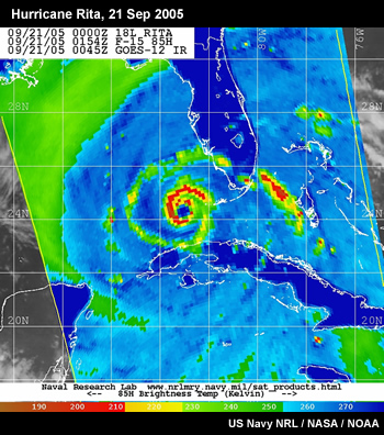
Continuing maintenance of the favorable environmental conditions for tropical cyclogenesis and intensification leads to further intensification into a more intense tropical cyclone with a symmetric structure and a clear eye (Fig. 8.9). Traditionally, vertical wind shear has generally been considered to have a negative effect on tropical cyclone intensification. An exception to this rule is the role of the TUTT in intensifying western North Pacific storms. New research is now challenging this view: vertical wind shear has been shown to intensify storms in a marginal thermodynamic environment.24,25,26 These storms must already be sufficiently intense to survive the initial disruption of their convection by the vertical wind shear, explaining why shear is still considered to be a negative effect on tropical cyclogenesis.
Regional differences also may provide the source of the forcing leading to this further intensification. For example, storms forming on the Northwest Shelf off the west coast of Australia may track parallel the coast for hundreds of kilometers. The warm waters of the "Northwest Shelf" provide the ideal environment for continued intensification of these storms until they either encounter the midlatitude westerlies (and their associated strong vertical wind shear) or a dry air intrusion from the Australian deserts disrupts the convective organization of the system.
8.2 Three-Dimensional Structure and Flow Balances »
8.2.2 Stages of a Typical Tropical Cyclone Lifecycle »
8.2.2.4 Severe Tropical Cyclone (supertyphoon, major hurricane)
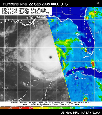
Relatively few tropical cyclones reach this status, characterized by peak sustained surface winds in excess of 50 m s-1 (Box 8-2, Fig. 8.10). Intensification to severe tropical cyclone requires that the storm remain over the open ocean, so storms forming close to land are less likely to reach such intensities. However, there are exceptions to every rule: the tropical cyclones off the Western Australian coast, described in the previous section, form and track relatively close to land; further, storms in the Bay of Bengal, Gulf of Mexico, and Western Caribbean have been observed to intensify rapidly into severe tropical cyclones. Wilma (2005, Box 8-3) is one such storm. Other historically significant severe tropical cyclones are reviewed in Boxes 8-3, 8-4, and 8-10.
Relatively few tropical cyclones reach this status, characterized by peak sustained surface winds in excess of 50 m s-1 (Box 8-2, Fig. 8.10). Intensification to severe tropical cyclone requires that the storm remain over the open ocean, so storms forming close to land are less likely to reach such intensities. However, there are exceptions to every rule: the tropical cyclones off the Western Australian coast, described in the previous section, form and track relatively close to land; further, storms in the Bay of Bengal, Gulf of Mexico, and Western Caribbean have been observed to intensify rapidly into severe tropical cyclones. Wilma (2005, Box 8-3) is one such storm. Other historically significant severe tropical cyclones are reviewed in Boxes 8-3, 8-4, and 8-10.
One limit on the intensity of storms in the SH is the relatively zonal nature of the mean flow. The SH has much smaller land masses and mountain ranges than the NH, providing less obstruction to the atmospheric flow. The result is more zonal mean midlatitude winds with the mean westerly zone being closer to the equator. In contrast, the many mountain ranges and large extents of the NH continents result in a large meridional component to the mean flow, which can steer tropical cyclones to much higher latitudes. The relative susceptibility of Japan (roughly 36°N) to tropical cyclone landfalls compared to, say, New Zealand (about 42°S) illustrates this point.
8.2 Three-Dimensional Structure and Flow Balances »
8.2.2 Stages of a Typical Tropical Cyclone Lifecycle »
8.2.2.5 The End of the Tropical Cyclone Lifecycle: Decay or Extratropical Transition (ET)
When a tropical cyclone moves into a hostile environment it will either decay (Fig. 8.11) or undergo extratropical transition. As might be expected, a hostile environment includes at least one of the following: strong vertical wind shear (in excess of 10-15 m s-1 over a deep layer), cool ocean temperatures under the storm core (less than 26°C), dry air intrusion, or landfall. Cool SST and strong shear are typical of a midlatitude environment, explaining why this region is generally thought to be a tropical cyclone graveyard. The hostile environment may unbalance the storm so that it ceases to be self-sustaining—and will decay—but intense storms may instead undergo transition into an extratropical cyclone (Section 8.5Section 8.5).
8.2 Three-Dimensional Structure and Flow Balances »
Box 8-3 Record Tropical Cyclone Intensity in the Eastern and Western Hemispheres
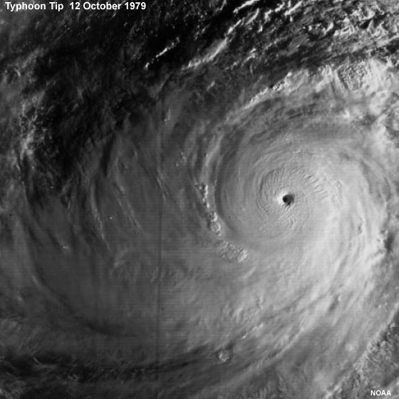
Supertyphoon Tip (1979) – The Most Intense Tropical Cyclone on Record
Supertyphoon Tip was legendary for its spatial extent as well as its intensity – most of the North Pacific basin appeared to be rotating! At its most intense, the minimum sea level pressure of Tip was measured at 870 hPa at 0353 UTC on 12 October 1979.27 The estimated maximum sustained (1-minute) surface wind was 85 m s-1 (305 km h-1).
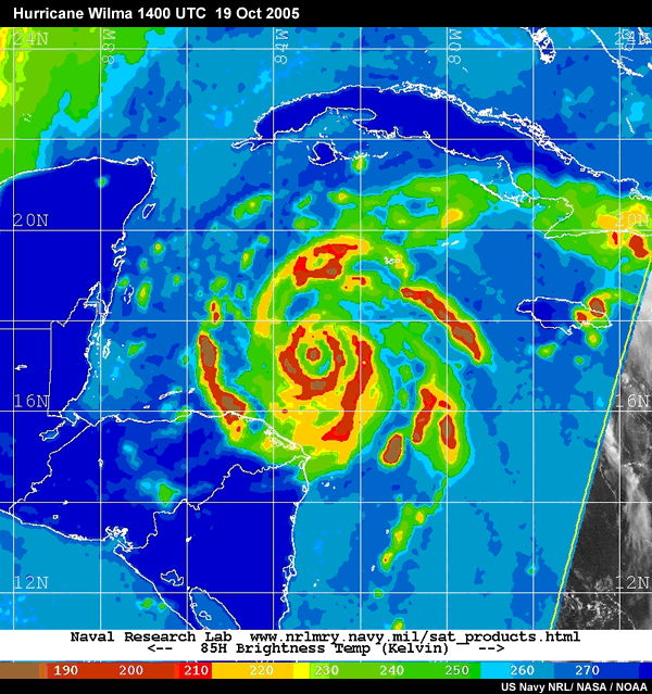
Major Hurricane Wilma (2005) – The Most Intense in the Western Hemisphere
Three days after forming in the northwestern Caribbean Sea and gradually intensifying, Wilma went through an unprecedented intensification cycle from 953 hPa to 901 hPa between 2310 UTC 18 October and 0433 UTC 19 October 2005: a rate of almost 10 hPa h-1! Around 1200 UTC 19 October 2005, Wilma attained its record-setting Category 5 intensity with maximum 1-minute 10-meter winds of 82 m s-1 (295 km h-1) with 882 hPa minimum central pressure—6 hPa lower than the previous record of 888 hPa in Hurricane Gilbert (1988). At peak intensity, Air Force reconnaissance measured its eye diameter to be only 3.7 km. Wilma was a Category 5 hurricane for a day. On 20 October the eye diameter expanded to 74 km and the peak winds dropped to 67 m s-1. Wilma maintained this now very large eye for most of the remainder of its lifecycle. Twenty-two fatalities were directly attributed to Wilma: 12 in Haiti, 1 in Jamaica, 4 in Mexico, and 5 in Florida.
8.2 Three-Dimensional Structure and Flow Balances »
8.2.3 Mass Balance Solutions and Scaling Considerations
Many investigators have considered the tropical cyclone in terms of a symmetric balanced vortex,28,29,30,31 yet inspection of this vortex reveals differing balance conditions in different regions of the vortex.11 In this section we explore the tropical cyclone vortex, identifying regions in which the balance constraint is cyclostrophic, gradient or even close to geostrophic, and then we introduce inertial stability and evaluate its spatial variation and evolution in the TC. Finally, we consider the three–dimensional, symmetric thermal wind balance.
8.2 Three-Dimensional Structure and Flow Balances »
8.2.3 Mass Balance Solutions and Scaling Considerations »
8.2.3.1 Geostrophic, Gradient and Cyclostrophic Wind Balances in the TC
An example of the close agreement between observations of rotational winds in Hurricane Diana (1984) and the corresponding gradients winds (calculated from the observed height field) is given in Fig. 8.12.11
The Rossby number is a nondimensional parameter that identifies the relative importance of the inertial and Coriolis terms in the Navier Stokes equations. It is defined by doing a scale analysis of these two terms and taking their ratio. The equation for the Rossby number is
 (1)
(1)where V is the scale speed, L is the scale distance and f is the Coriolis parameter.
Another interpretation of the Rossby number is that it gives the ratio of the vorticity of the flow to the Earth's vorticity, f. The magnitude of the Rossby number gives insight into the type of force balance dominating:
 (2)
(2)Thus, calculation of the Rossby number for various regions of a typical tropical cyclone will tell us about the important force balances in this region. We now consider three distinct regions of the storm: the eye, the area inside the gale force wind radius, and the "outer" storm (Fig. 8.13).
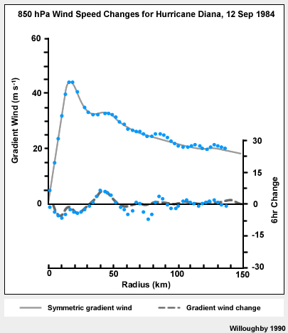
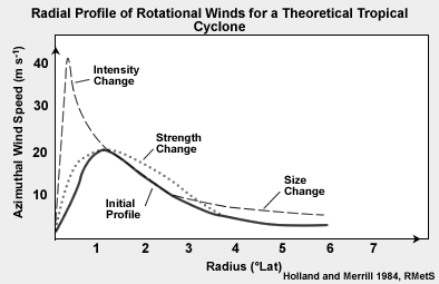
Based on Figures 8.12 and 8.13, typical power of 10 values for wind speed and spatial scale for the three regions of this tropical cyclone are:
| Eye | V ~ 10 m s-1 | L ~ 104 m |
| Storm Strength | V ~ 10 m s-1 | L ~ 105 m |
| Outer | V ~ 1 m s-1 | L ~ 106 m |
These numbers correspond to winds of 10 ≤ V < 100 m s-1 over a spatial scale of ~10 km for the eye, V > 10 m s-1 over a spatial scale ~1000 km for the storm-force wind area, and V < 10 m s-1 over a spatial scale >1000 km for the outer region of the storm. Recalling that a degree of latitude is roughly 100 km, these numbers are consistent with Fig. 8.13.
To calculate the Rossby number, we still need a value for the Coriolis parameter, f. Assuming a reasonable latitude of 15° gives f =4×10⁻⁵. Again, for an order of magnitude analysis, we round this value of f to the nearest power of 10. Thus, we will use f~ 10-5 s-1.
Now let’s calculate the Rossby number for each region:
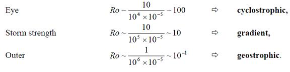
So we see that different balances can apply to the different regions of a tropical cyclone.22,23
Use Fig. 8.13 to select typical numbers (not orders of magnitude) for wind speed and spatial scale for each of the three regions (eye, storm–force, outer) for both an intense (40 m s-1; long dash) and a weak (20 m s-1; solid line) tropical cyclone. Use f~ 10-5 s-1 as before. In both storm analyses take (a) 15 m s-1 for the "strength" wind value and (b) 500 km for the outer wind radius.
Compare the resulting values for Rossby number for each storm in each region. Now compare these values with the order of magnitude analysis given above and decide whether the fundamental balances in each region would change with changing intensity.
Click "done" for feedback.
Feedback:
Using Fig. 8.13 as a guide, typical values for wind speed and spatial scale in the three regions for each tropical cyclone are:
| Eye | V ~ 40 m s-1 | L ~ 50 km = 5 x 10³ m |
| Storm Strength | V ~ 15 m s-1 | L ~ 150 km = 1.5 x 10⁵ m |
| Outer | V ~ 10 m s-1 | L ~ 500 km = 5 x 10⁵ m |
The Rossby numbers for each region of the 1st example, the 40 m s-1 tropical cyclone are
| Eye | V ~ 20 m s-1 | L ~ 120 km = 1.2 x 10⁴ m |
| Storm Strength (as above) |
V ~ 15 m s-1 | L ~ 150 km = 1.5 x 10⁵ m |
| Outer | V ~ 4 m s-1 | L ~ 500 km = 5 x 10⁵ m |
The Rossby numbers for each region of the 2nd example, the 20 m s-1 tropical cyclone are
We can glean a number of interesting results from these analyses:
- The balance structures of different storms vary with radius.
- The 20 m s-1 storm agrees with our order of magnitude scale analysis in all regions.
- The gradient wind region extends further for the 40 m s-1 storm than the 20 m s-1 storm. This means that we can expect different balances to occur at different radii for tropical cyclones with different radial structure (i.e. cyclones whose rotating winds change differently as you move out from their center).
The horizontal wind balances just discussed are not the only balance constraints operating in a symmetric, steady state tropical cyclone. The inertial stability and the thermal wind of the vortex provide information about the vertical wind shear of the balanced flow associated with the storm and its resistance to outside influences.
8.2 Three-Dimensional Structure and Flow Balances »
8.2.3 Mass Balance Solutions and Scaling Considerations »
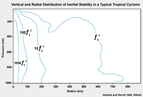
8.2.3.2 Inertial Stability Variations in a TC
Inertial stability, symbolized as I, is a measure of the resistance of a symmetric vortex to forcings acting to change its structure. Examples include convective heating or other weather systems.
For a tropical cyclone, the horizontal winds dominate the flow and the inertial stability is defined by:
 (3)
(3) where, ζ is the relative vorticity, fo is the local Coriolis parameter (a constant at the center of rotation), and v/r is the relative angular velocity. Clearly, the inertial stability will increase proportionally with the relative vorticity, Coriolis parameter, and wind speed, and will increase as radius decreases. Thus, a storm that is contracting and increasing in intensityd will rapidly increase its inertial stability, increasing its resistance to horizontal forcing by external weather systems.33,34 Also, for a given radius and latitude, as wind speed increases the inertial stability at that location increases. This means that we expect the inertial stability to vary with location in the tropical cyclone (Fig. 8.14).
The anticyclonic outflow aloft has very weak absolute vorticity (ζ has the opposite sign to f and the rotational winds are weak; the signs of both ζ and v act to reduce the effect of the Coriolis parameter on I). Thus, while an intense symmetric cyclone is more protected from influences that might weaken it, its strong inertial stability does not extend to the tropopause. This means that upper tropospheric weather systems may still act to weaken the storm. Further, inertial stability cannot protect the storm from surface influences such as cool SST. This understanding of inertial stability helps explain why tropical cyclones of increasing intensity are more likely to survive adverse environmental influences, but their "Achilles' heel" is the anticyclonic outflow.
The concept of inertial stability can be illustrated by a thought experiment in a swimming pool. Perhaps some of you have done this. If you walk around and around a circular swimming pool you can force the water into rotation in the same direction. Once the water is in motion, will it be easy or difficult to (a) walk into the center of the pool; and (b) to turn around and walk the other way around the edge of the pool (against the current)?
If you have not done this before, give it a try – how often to you get to play and call it meteorology research?
Feedback:
Inertial stability illustrated in a swimming pool: It will be difficult both to walk into the center of the pool and to turn around and walk against the current. The inertial stability of the rotating water resists motions across the flow and against the flow.
Inertial stability evolution due to a contracting eyewall: What happens to the inertial stability (a) of the eye; and (b) to the flow at the "old" eye radius? Use the above equation to guide your thinking.
Feedback:
Inertial stability evolution due to a contracting eyewall: (a) As the eyewall contracts the wind speed increases, but the radius decreases (we do not know what is happening to f, so we assume that it remains constant). As a result of the radius decreasing, we see that inertial stability of the contracting eye increases. (b) At the "old" eye radius, the radius is unchanged while the wind speed has decreased. Thus, the inertial stability at this radius decreases.
d For example, during an eyewall replacement cycle (Section 8.4.5.3).
8.2 Three-Dimensional Structure and Flow Balances »
8.2.3 Mass Balance Solutions and Scaling Considerations »
8.2.3.3 The Thermal Wind
A symmetric tropical cyclone is in approximate thermal wind balance. The thermal wind is defined as the difference between the geostrophic wind at two vertical levels
 (4)
(4)where pA and pB are the pressures “above” and “below” so that pA < pB. Thus, the thermal wind represents the vertical wind shear of the geostrophic wind. For geostrophic flow, the thermal wind balance is written as
 (5)
(5)where pA and pB bound the layer in which the mean temperature gradient,  , is calculated and zA and zB are the physical heights of these pressure layers. Therefore, by using the horizontal temperature gradient at the level of the warm core and the surface wind structure, we can infer the three–dimensional symmetric wind field of the cyclone.
We can deduce the change of the winds with height using the thermal wind. For a tropical cyclone, the winds are strongest at the surface and decrease with height; from Equation (5) we can show that this corresponds to a warm temperature anomaly associated with the storm and that this anomaly is maximum in the upper troposphere. As a result, tropical cyclones may be referred to as "warm–cored." Conversely, a midlatitude storm has its strongest winds aloft (typically near the tropopause); using Equation (5) again, these systems can be shown to be "cold–cored" in the upper troposphere.
The Cyclone Phase Space (CPS)35 is a diagnostic that utilizes the thermal wind to document the structure of meso-synoptic cyclones concisely. CPS diagnostics are used to distinguish different phases of the development in the lifecycle of a tropical cyclone, for example, the onset and completion of the transitions from subtropical to tropical cyclones23 and from tropical to extratropical cyclones36 (Section 8.5).
The Cyclone Phase Space(CPS)35 is a diagnostic that utilizes the thermal wind to document the structure of meso-synoptic cyclones concisely. CPS diagnostics are used to distinguish different phases of the development in the lifecycle of a tropical cyclone, for example, the onset and completion of the transitions from subtropical to tropical cyclones23 and from tropical to extratropical cyclones36 (Section 8.5).
http://moe.met.fsu.edu/cyclonephase/help.html
Realtime CPS diagnostics for operational models and microwave satellite data (where available),
http://moe.met.fsu.edu/cyclonephase/
Diagnosing and Forecasting ET: Hurricane Michael (2000),
http://www.meted.ucar.edu/norlat/ett/michael/
8.2 Three-Dimensional Structure and Flow Balances »
8.2.4 Post-landfall Structure
Changes in the tropical cyclone boundary layer when the storm crosses the coaste — that is, when the storm "makes landfall" (e.g., Fig. 8.15) — critically influence the subsequent distribution of significant weather due to that tropical cyclone. With rare exceptions (ships at sea, storms that stay just offshore, oil platforms and other structures), the major impacts from a tropical cyclone occur at, and after, landfall. Thus, we should consider post-landfall structure changes.
Two major changes of the storm environment at landfall cause it to weaken: loss of the ocean energy source and increased friction. The resulting changes in storm structure lead to a redistribution of the significant weather associated with the storm. Each of these processes is worthy of further discussion.
Evaporation (latent heat flux) and heat transfer (sensible heat flux) from the ocean surface warm and moisten the tropical storm boundary layer, providing energy to feed the clouds that drive the tropical cyclone. Hence, when the storm loses this energy source it begins to weaken. We can picture the outcome of this weakening by making use of thermal wind balance of a symmetric vortex: the lack of a moisture source over land weakens the convection and associated subsidence in the eye weakens the upper tropospheric warm core, raising the central pressure of the storm. This increase in the central pressure leads to weaker pressure gradient and weaker gradient wind.
Surface friction effects on the atmosphere increase significantly after landfall. The ocean surface has less drag on the air than the solid land so the storm is able to sustain stronger peak surface winds over water. Land surfaces have a greater "roughness" (due to topography and natural and man-made structures) which leads to greater frictional drag and weaker winds.
These two mechanisms for slowing the surface winds take time to act and their influence will change with new changes to the surface. Any change in surface roughness (landfall or change in land use) will result in the formation of a new "internal" boundary layer that is in balance with the new surface. The (new) internal boundary layer will form in the timescale of an inertial period of the storm, which is about an hour in the strong wind part of the storm.
The ultimate impact of landfall on the surface winds depends on a variety of factors. For example, if the storm comes ashore in the coastal plains and river deltas of the Gulf of Mexico, the frictional effects will be much less than if it makes landfall in a mountainous place like Taiwan or Central America. Land use also matters: all else being equal, a heavily built-up or forested area will have a larger frictional effect than a swamp—and evaporation of moisture from the swamp may delay weakening or even cause the storm to temporarily reintensify.37 A storm is generally modified differently by passage over an island compared to a continental land mass. For example, the loss of surface energy source and the increased friction will have less impact for a tropical cyclone moving over an island than if it moved completely over land. The size of the island and its topographic scale will cause a range of impacts on the storm.
While post-landfall structure changes generally lead to a decrease in the near-surface wind speeds as described above, the roughness of the terrain can contribute to regions in which the gusts are stronger than the frictionally-reduced surface winds.
The final effect of landfall on the tropical cyclone is the redistribution of its significant weather: weakening the surface pressure gradient causes the boundary layer convergence zone to shift outwards, leading to a redistribution of the convection and development of broad regions of stratiform rain (which feeds off the moisture transported onshore with the storm). The strong moisture gradient between the storm and its landfall environment coupled with the vertical wind shear profile can create the ideal conditions for tornadic thunderstorms. Tornadoes generated with the passage of Hurricane Ivan (2004) caused major damage in Florida, even though the storm made landfall further west. Lightning generated in the unstable coastal zone can also create a hazard (generally just offshore) to the population near the coast.38,39
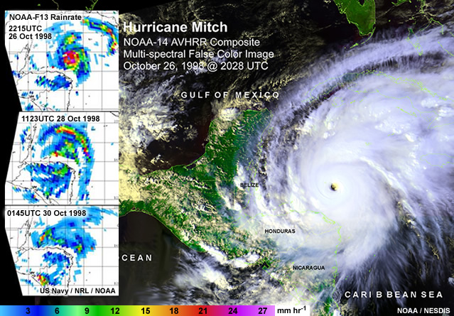
As with the frictional weakening of the storm, topography can play a role in these weather-related impacts: the topographic enhancement of the already intense rainfall associated with the storm. Hurricane Mitch (1998) is a terrible example of this combination of very intense rain with unstable mountain slopes leading to large-scale mudslides and loss of life (Box 8-4).
As with the frictional weakening of the storm, topography can play a role in these weather-related impacts: the topographic enhancement of the already intense rainfall associated with the storm. Hurricane Mitch (1998) is a terrible example of this combination of very intense rain with unstable mountain slopes leading to large-scale mudslides and loss of life (Box 8-4).
Helene (2000), http://www.nhc.noaa.gov/2000helene.html
Erin (2007), http://www.nhc.noaa.gov/pdf/TCR-AL052007_Erin.pdf
e From a forecasting perspective, "landfall" does not occur until the center (minimum pressure and winds) of the tropical cyclone has crossed the coast (Avila, pers. comm. 2008).
8.2 Three-Dimensional Structure and Flow Balances »
Box 8-4 Hurricane Mitch (1988): A Devastating Storm in Central America
Over 10,000 fatalities were attributed to Hurricane Mitch, predominantly from flooding in Honduras and Nicaragua due to its slow movement and topographic enhancement of its rainfall. For a week the overall storm motion was less than 2m s-1 (4 kts). Heavy rains on unstable hillsides caused large-scale mudslides, which buried or swept away entire villages. Synoptic reports had a maximum of 911 mm (35.89 in) for 25-31 October but data were missing from many stations. Satellite-based estimates ranged from 900-1500 mm. Mitch is the strongest recorded October hurricane in the Atlantic (records began in 1886), with minimum central pressure of 905 hPa (tying Hurricane Camille of 1969) and maximum wind speed estimated at 80 m s-1 (290 km h-1, 155 kts, 179 mph).
Very few Atlantic storms have been as devastating as Mitch. Hurricane Fifi (1974, Honduras), a 1930 hurricane (Dominican Republic) and Hurricane Flora (1963, Haiti and Cuba) are all recorded to have caused around 8,000 fatalities, as was the Galveston Hurricane of 1900. However, the largest confirmed loss of life due to a hurricane in the Western Hemisphere was due to The Great Hurricane of October 1780, which is estimated to have caused the deaths of about 22,000 people, with around 9,000 lost in Martinique, 4,000-5,000 in St. Eustatius, and over 4,300 in Barbados.40 Thousands of deaths also occurred offshore.
http://www.nhc.noaa.gov/pastdeadly4.shtml
NHC report on Hurricane Mitch, http://www.nhc.noaa.gov/1998mitch.html
NCDC, storm review, each country's damage,
http://lwf.ncdc.noaa.gov/oa/reports/mitch/mitch.html
Mitch Rainfall, http://www.nrlmry.navy.mil/sat_training/tropical_cyclones/ssmi/rain/index.html
Hurricane Mitch Satellite Time Series, http://www.osei.noaa.gov/mitch.html
Hurricane of 1780, http://www.jamaica-gleaner.com/pages/history/story008.html
8.3 Tropical Cyclogenesis
What is tropical cyclogenesis? Surprisingly, there is no single answer to this question. Operational forecast centers responsible for issuing tropical cyclone watches and warning define genesis as observed sustained mean surface winds (averaging time is dependent on region) in excess of tropical storm force (17 m s-1; 60 km h-1; 33 knots). While this is a readily applied and unambiguous criterion for tropical storm formation, it is not particularly helpful in understanding the processes leading to genesis. However, implicit in this operational genesis criterion is the expectation that the tropical storm will continue to develop from this point forward; that is, that the storm will become self-sustaining. This is the definition of genesis that we will use here: tropical cyclogenesis has occurred when the tropical storm has become self-sustaining and can continue to intensify without help from its environment (external forcing).
8.3 Tropical Cyclogenesis »
8.3.1 Necessary Conditions for the Formation of a Tropical Cyclone
Six features of the large-scale tropics were identified by Gray (1968)41 as necessary, but not sufficient conditions for tropical cyclogenesis:
| (i) | sufficient ocean thermal energy [SST > 26°C to a depth of 60 m], |
| (ii) | enhanced mid-troposphere (700 hPa) relative humidity, |
| (iii) | conditional instability, |
| (iv) | enhanced lower troposphere relative vorticity, |
| (v) | weak vertical shear of the horizontal winds at the genesis site, and |
| (vi) | displacement by at least 5° latitude away from the equator. |
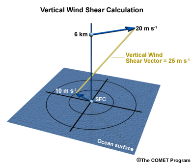
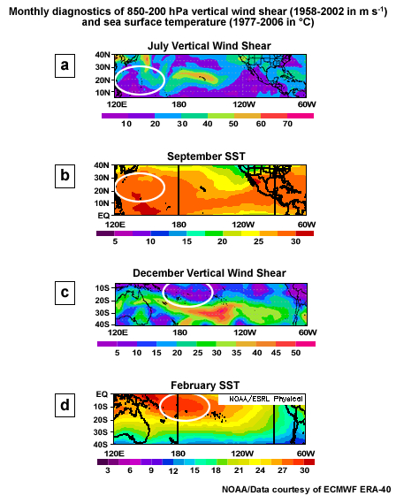
The first three thermodynamic parameters measure the ability to support deep convection—criteria that have been identified as seasonal indicators of genesis potential. The latter, dynamical parameters, such as vertical wind shear (Fig. 8.16), measure the daily likelihood of genesis.42 In recent years, a number of tropical cyclones have remained within 5° latitude of the equator,43 suggesting a need to relax this constraint. Many, but not all, of those near-equatorial systems had very small spatial scale. Locations where conditions (i) and (v) are satisfied are highlighted in Figure 8.17.
“Necessary but not sufficient” means that all of these conditions must be present simultaneously before tropical cyclogenesis can occur, but even if all of these conditions are met, tropical cyclogenesis may not occur. Thus, the necessary, but not sufficient, criteria for tropical cyclogenesis may be summarized as the ability to support deep convection in the presence of a low-level absolute vorticity maximum. The low-level vorticity maximum reduces the local Rossby radius of deformationf focusing the convective heating locally.
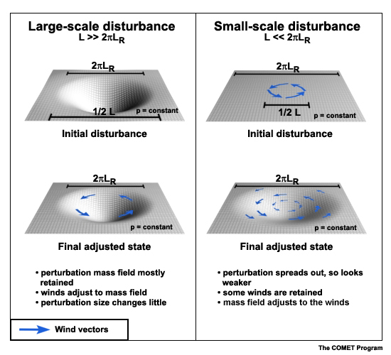
The ability of the initial convection to survive for many days depends on its vorticity, stability, and depth—defined by the Rossby radius of deformation, LR. The Rossby radius, LR, is the critical scale at which rotation becomes as important as buoyancy. When the disturbance size is wider than LR, it persists; systems that are smaller than LR will disperse (Fig. 8.18). LR is inversely proportional to latitude so it is very large in the tropics. However, the high vorticity in tropical cyclones reduces the Rossby radius and enables tropical cyclones to last for many days and even weeks.
The ability of the initial convection to survive for many days depends on its vorticity, stability, and depth—defined by the Rossby radius of deformation, LR. The Rossby radius, LR, is the critical scale at which rotation becomes as important as buoyancy. When the disturbance size is wider than LR, it persists; systems that are smaller than LR will disperse (Fig. 8.18). LR is inversely proportional to latitude so it is very large in the tropics. However, the high vorticity in tropical cyclones reduces the Rossby radius and enables tropical cyclones to last for many days and even weeks.
http://www.australiasevereweather.com/cyclones/2002/summ0112.htm
f For a weather system with large relative vorticity, such as a tropical cyclone, LR can be generalized as

where ζ is the vertical component of the relative vorticity, N is the Brunt Väisäla frequency, H is the depth of the system and fo is the Coriolis parameter.
8.3 Tropical Cyclogenesis »
8.3.2 Dynamic Controls on Genesis in the Monsoon Trough Environment
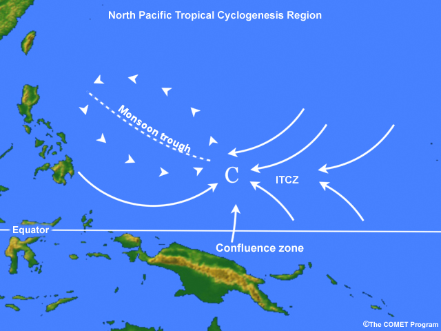
In most basins, the monsoon trough is the most common region for genesis, so we begin with a review of the controls on tropical cyclogenesis in the monsoon trough environment. A new way of looking at the tropical western North Pacific is to partition its large–scale tropical environment into a monsoon trough zone and an ITCZ zone, separated by a confluence zone (Fig. 3.42). The monsoon trough zone is characterized by the near–equatorial seasonal westerly winds and enhanced rainfall. Lower tropospheric vorticity in the monsoon trough zone is derived from the cyclonic circulation that results from the incursion of the monsoon westerlies. In contrast, the ITCZ zone is dominated by trade easterlies throughout; these low–level easterlies converge in the ITCZ convective trough. The transition zone between the near-equatorial monsoon westerlies and ITCZ trade easterlies is known as the confluence zone. This combination of features—monsoon trough, confluence zone, and ITCZ—will be referred to here as the monsoon region.
8.3 Tropical Cyclogenesis »
8.3.2 Dynamic Controls on Genesis in the Monsoon Trough Environment »
8.3.2.1 Alternative Monsoon Trough Modes
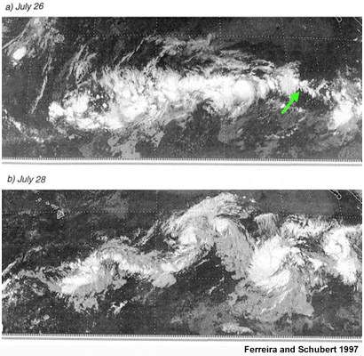
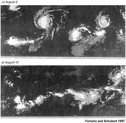
Three potential paths to tropical cyclogenesis in the monsoon region of the western North Pacific have been newly identified:44 two distinct modes of monsoon trough breakdown18 and monsoon gyres.45 Satellite images show an example of the monsoon trough breakdown and subsequent tropical cyclone genesis (Fig. 8.19).
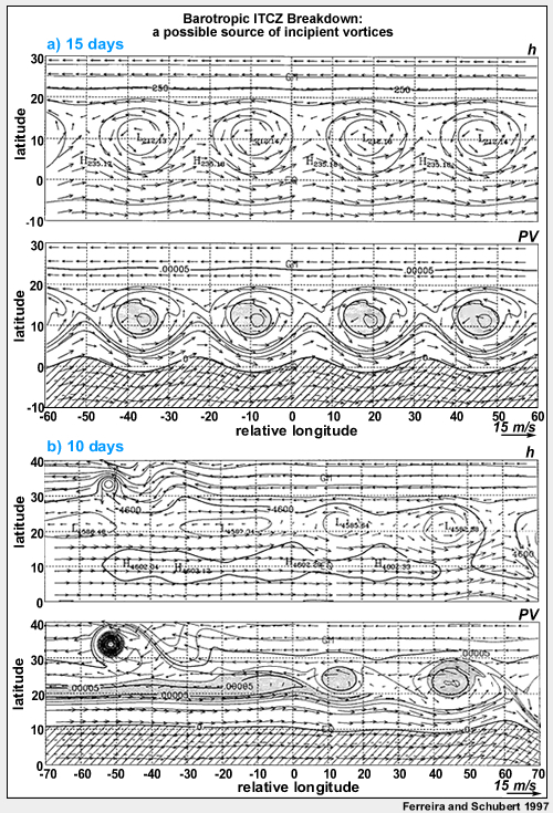
A straightforward potential vorticity (PV) model for the Hadley cell provides ample evidence that the continuous PV source associated with convection in the ITCZ will act to destabilize and break down the ITCZ periodically18 through combined barotropic-baroclinic instability. Two outcomes can result from the barotropic mode of ITCZ instability and associated monsoon trough breakdown: formation of a group of several tropical cyclones, or re-symmetrization and development of one, larger, tropical cyclone19 (Fig. 8.20). As the figure shows, the shape of the initial PV strip used to characterize the ITCZ, as well as the presence of another cyclone, affect which mode of breakdown occurs. The presence of an additional cyclonic vortex in the ITCZ sped its breakdown.
The monsoon gyre is defined as a closed, symmetric circulation at 850 hPa with horizontal extent of 25° latitude that persists for at least two weeks.45 This circulation is accompanied by abundant convective precipitation around the south-southeast rim of the gyre. The gyre has similar scale and structure to the second mode of the barotropic monsoon trough breakdown and genesis just described (Fig. 8.20b). We cannot yet say whether the gyre is this monsoon breakdown or a distinct path to genesis, however two studies44,46 of the frequency of different paths to genesis in the monsoon regime suggest that the gyre is a relatively rare path to genesis.
8.3 Tropical Cyclogenesis »
8.3.2 Dynamic Controls on Genesis in the Monsoon Trough Environment »
8.3.2.2 Equatorial Waves
Twin tropical cyclones that straddle the equator47 at formation have a flow structure suggestive of equatorial Rossby waves48,49 (Fig. 8.21, Section 4.1.2).
Twin tropical cyclones that straddle the equator47 at formation have a flow structure suggestive of equatorial Rossby waves48,49 (Fig. 8.21, Section 4.1.2).
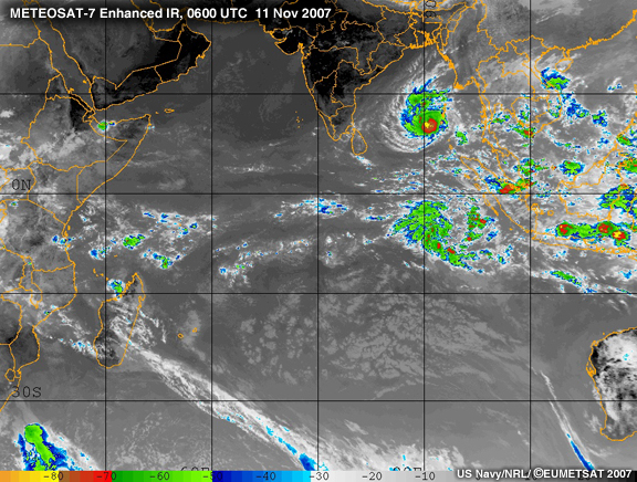
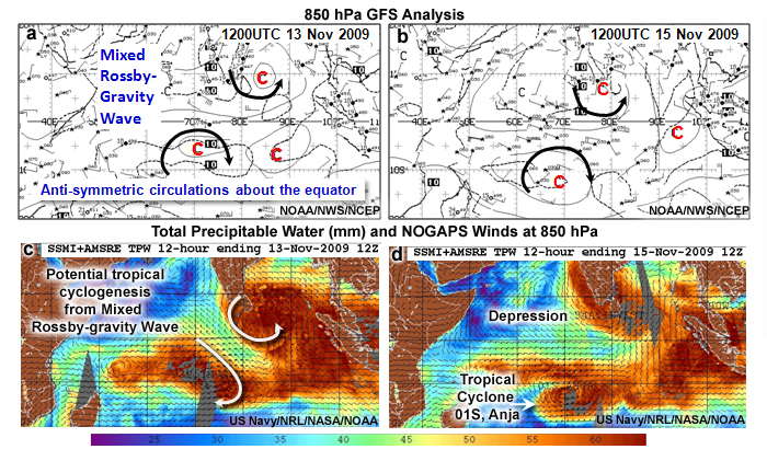
While the case depicted in Fig. 8.21 is evidence that equatorial Rossby waves equatorial Rossby waves may initiate genesis, others argue that the shorter wavelength mixed Rossby-gravity waves mixed Rossby-gravity waves are also important (Fig. 8.22 and Fig. 9.34).50
In the process of tropical cyclogenesis from an equatorial wave, a region of active convection forms on the northwest side of a near-equatorial wave trough (in the region of maximum low-level convergence for a mixed Rossby-gravity wave). This convective region moves away from the equator and may eventually develop into a tropical storm (Fig. 8.21, Fig. 8.22). The ultimate formation of a tropical depression is attributed to enhanced Ekman pumping51 in the evolving depression (consistent with CISK or free ride development).52,53,54
Numerical modeling studies using barotropic models have examined the non-linear evolution of wave activity over the western North Pacific in association with the background confluent flow (recall confluent zone in Fig. 8.19). If waves with wavelengths near 2000 km are continuously generated upstream (to the east in the deep tropics), their energy will accumulate in the monsoon confluence zone. This results in a scale contraction of short Rossby waves leading to the formation of an incipient vortex on the right spatial scale to become a tropical cyclone. This process may even result in a sequence of vortex formations in the confluent eastern end of the western North Pacific monsoon region.
The western North Pacific does not hold the monopoly on equatorial waves: preferential wave growth also occurs in the dynamically unstable and convectively active eastern Pacific ITCZ.17 Two hypotheses have been advanced to explain the maintenance of the mean meridional PV gradient here: either convectively-forced PV generation; or cross equatorial advection of absolute vorticity driven by high cross-equatorial pressure gradients in the ITCZ region.55 In the second scenario, convection is a consequence of the dynamic instability, rather than its driver, consistent with the temporal lag between the convective heating and the peak in the PV gradient.56
An unexpected path to genesis was revealed in an idealized study of the evolution of a Rossby wave advected in easterly flow across a mountain range (representing the Sierra Madres of Mexico). The interaction led to the development of a lee trough and a secondary vorticity maximum that propagated downstream with period about 5 days.21 Both the lee trough and secondary vorticity maximum are potential locations for tropical cyclogenesis.57 Thus, development of this lee trough can serve a similar role in genesis to the monsoon confluence zone of the western North Pacific.
The seasonality of tropical cyclogenesis has been related to the convective potential of the region being considered, while dynamical factors contribute to the daily potential for genesis.42 Regions of observed tropical cyclogenesis are associated with preferred wave growth (along the equator or the "dynamic equator" associated with the ITCZ) or the monsoon region. The unifying dynamical characteristic of these regions is a sign reversal of the meridional gradient of the large-scale PV. This PV gradient reversal satisfies the Charney-Stern condition for dynamic instability.58
8.3 Tropical Cyclogenesis »
8.3.2 Dynamic Controls on Genesis in the Monsoon Trough Environment »
8.3.2.3 Tropical Cyclogenesis Associated with the TUTT
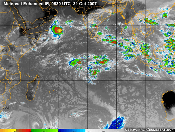
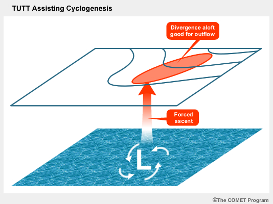
In the monsoon confluence zones, genesis may be initiated through easterly waves that propagate into the region. The genesis process may be due to the interaction between an easterly wave and a Tropical Upper Tropospheric Trough (TUTT). The TUTT is a meso-synoptic upper cold low that has been linked to genesis in the western North Pacific and North Atlantic. It can be identified on satellite imagery as a clear region with widely scattered, small convective cells. The presence of an equatorial wave17,21,50,57 or an easterly wave and the possible interaction with the TUTT59,60 will locally enhance low-level convergence and thus moist convection, providing a favorable environment for tropical cyclogenesis (Fig. 8.23). Tropical cyclones have also been proposed as a mechanism for the formation of TUTT cells and that this formation is preconditioned by the large-scale environmental shear. Thus, the TUTT could be a consequence, rather than a driver, of tropical cyclogenesis.
8.3 Tropical Cyclogenesis »
Box 8-5 They Lived to Tell the Tale!
The roots of this story are a little unclear, but one version states that a group of pilots, including Lt Col Joe Duckworth, were comparing the abilities of their planes. At that time, Duckworth was on assignment training pilots to fly AT-6 aircraft in bad weather. Duckworth maintained that his aircraft could even survive a hurricane. On a dare, he and navigator Ralph O'Hair flew into a hurricane in the Gulf of Mexico. This was the first recorded intentional flight into a tropical cyclone!
According to National Weather Service records, Duckworth and O'Hair must have flown into the first recorded storm for 1943 (storms were not named until 1950). This storm later made landfall in Texas as a Category 2 hurricane.
The tradition begun by Duckworth and O'Hair continues to this day: the 53rd Weather Reconnaissance Squadron of the Air Force Reserve (commonly known as the "Hurricane Hunters") and the NOAA Corps continue operational and research flights into hurricanes today.
Hurricane Hunters, http://www.hurricanehunters.com/
(Air Force Reserve 53rd Weather Reconnaissance Squadron,
403rd Wing, Keesler Air Force Base http://www.keesler.af.mil/)
NOAA Aircraft Operations Center, http://www.aoc.noaa.gov/index.html
NOAA Corps, http://www.noaacorps.noaa.gov/
8.3 Tropical Cyclogenesis »
8.3.3 Mesoscale Influences on Tropical Cyclogenesis
In this discussion, we examine the mesoscale features in the environment that can generate an incipient tropical cyclone vortex and sustain it until genesis takes place. Mesoscale influences on tropical cyclone formation include effects contributing to (or limiting) the creation of the incipient vortex or disturbance and the eventual survival of that vortex.
Monsoon depressions,61 African easterly waves,21 and subtropical cyclones62 have long been understood to provide source disturbances from which, under appropriate thermodynamic conditions, a tropical cyclone could develop. While the tropical eastern Pacific is widely recognized as being a very active region of tropical cyclogenesis, explanations for many of the paths to tropical cyclogenesis in this region have only been forthcoming in the last decade.
8.3 Tropical Cyclogenesis »
8.3.3 Mesoscale Influences on Tropical Cyclogenesis »
8.3.3.1 African Easterly Waves (AEW)
African easterly waves (Fig. 8.24) initiate tropical cyclogenesis in both the North Pacific and North Atlantic Oceans. They form over the African continent during the monsoon season. Easterly waves are well-defined wave perturbations with periods of roughly 3–5 days and spatial scale about 1000 km. They occur as waves with maximum amplitude close to the level of the African Easterly Jet (AEJ) and low-level maximum amplitude north of the jet. They move westward at speeds of 7–8 m s-1.
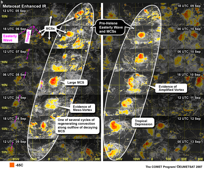
Mesoscale convective systems move with and through the synoptic-scale AEWs (Fig. 8.24b). Some tropical cyclones, such as Alberto (2000), began as AEW-MCS systems that initiate near the mountains of East Africa (the Darfur Mountains and Ethiopian Highlands) and move westward while undergoing cycles of regeneration of convection. A few of these systems evolve into tropical cyclones close to the African coast, e.g., Cindy (1999) and Helene (2006); (see Fig. 8.24b for images of Helene). The swirling cloud pattern at 1200 UTC 8 September and 1800 UTC 10 September (Fig. 8.24b) indicate the presence of a mesoscale convective vortex, a feature that sometimes forms in the stratiform region of decaying MCSs. The pre-Helene vortices appear to amplify over the continent within the AEW structure, a strong vortex emerges from the continent, and tropical cyclogenesis occurs soon after. The observations support the notion that mesoscale convection is a source of potential vorticity for tropical cyclogenesis. The interaction of the vorticity associated with AEWs and the mesoscale vorticity associated with MCSs is being studied in order to differentiate between strong and weak AEWs and the implications for tropical cyclogenesis. Mesoscale influences on tropical cyclogenesis are explored further in Section 8.3.3.3.
Mesoscale convective systems move with and through the synoptic-scale AEWs (Fig. 8.24b). Some tropical cyclones, such as Alberto (2000), began as AEW-MCS systems that initiate near the mountains of East Africa (the Darfur Mountains and Ethiopian Highlands) and move westward while undergoing cycles of regeneration of convection. A few of these systems evolve into tropical cyclones close to the African coast, e.g., Cindy (1999) and Helene (2006); (see Fig. 8.24b for images of Helene). The swirling cloud pattern at 1200 UTC 8 September and 1800 UTC 10 September (Fig. 8.24b) indicate the presence of a mesoscale convective vortex, a feature that sometimes forms in the stratiform region of decaying MCSs. The pre-Helene vortices appear to amplify over the continent within the AEW structure, a strong vortex emerges from the continent, and tropical cyclogenesis occurs soon after. The observations support the notion that mesoscale convection is a source of potential vorticity for tropical cyclogenesis. The interaction of the vorticity associated with AEWs and the mesoscale vorticity associated with MCSs is being studied in order to differentiate between strong and weak AEWs and the implications for tropical cyclogenesis. Mesoscale influences on tropical cyclogenesis are explored further in Section 8.3.3.3.
While African easterly waves tend to weaken and lose their convection in the central Atlantic, they are often reinvigorated as they pass through the Caribbean, gaining sufficient energy to complete their trek into the eastern Pacific. Indeed, tropical cyclone developments for the 1991 eastern Pacific season were preferentially downstream of inertially unstable zones (such as the Caribbean) consistent with the continued progression of equatorial waves across the Western Hemisphere tropics.56
Easterly waves form in an environment similar to the first “multiple storm formation” mode of genesis pictured in Fig. 8.20 (upper panels), giving us confidence that this barotropic model captures the important physics of genesis here. So the multiple storm formation mode of genesis appears to be present in the African monsoon. Since other monsoon regions have very similar PV and convection structures,63 we expect that Africa should not be a unique region for easterly wave formation.18 This suggests that similar disturbances could also be generated in the Australian monsoon. Are easterly waves African then, or are they an international phenomenon?
A study assessing the potential for easterly wave formation in Australia compared to Africa63 found a 2–6 day peak in the variance of the African monsoon [identified by outgoing longwave radiation (OLR) and low-level winds] consistent with easterly wave activity,64 but no corresponding peak in the Australian data even if the criteria were relaxed.
What could cause the lack of easterly wave activity in Australia? (Type your response in the box below.)
Feedback:
Three possible reasons for the lack of easterly waves in Australia have been suggested so far:63,65 (1) the extent of Australian monsoon (PV gradient) region is only 60% of the African; (2) the lack of topography in Australia could lead to a weaker easterly jet; (3) or the stability of the Australian flow pattern damping out the waves.
So it looks, for now, like Africa is unique as a source for easterly waves.
8.3 Tropical Cyclogenesis »
8.3.3.2 Development from Subtropical Storms
Surprisingly, the role of subtropical storms in tropical cyclogenesis was hardly recognized until the last decade when a number of studies have explored this path to genesis for North Atlantic tropical cyclones.42,66,67,68 This slow recognition is exemplified by the fact that subtropical cyclones have often been used as a 'catch-all' category for different types of ambiguous storms, with forecasters calling them many different things including names like "neutercane". As a result of impacts from subtropical cyclones in the Atlantic, in 2002, the US National Hurricane Center began naming those storms from the same list as tropical cyclones are named.
Tropical cyclone formation from a subtropical storm requires that a deep warm-cored cyclone is created from a shallow, mid-level vortex (cold–cored in the lower-troposphere).16,66,67,69 The process of "tropical transition" of the subtropical cyclone into a tropical cyclone (Fig. 8.25) begins when a deep cold core trough (black +) in the upper westerlies approaches a low-level baroclinic zone — either a surface front over warm water, or a sharp SST gradient with warm water equatorward (e.g. the Gulf Stream). If the upper trough breaks off from the westerlies (a Rossby wave break)68 and becomes a cut-off low, its scale and speed of motion are favorable for the genesis of a subtropical storm. If the upper tropospheric cut-off low grows baroclinically, a reflection of the upper PV anomaly may develop near the surface (grey +). The resulting low–level baroclinic wave may serve to organize and focus the convection prevalent over warm (SST > 26°C) water.
The mid-level vortex must build down toward the surface to generate the surface inflow and increased surface fluxes needed for subsequent development.70,54 In an unstable environment, ascent into the mid-level vortex can force convection. The resulting convective heating leads to diabatic cyclonic PV generation below the level of maximum heating, thus building the vortex down to the surface.67 The cyclonic surface winds generate surface fluxes that increase the θe of air inflowing towards the nearly saturated core of the developing system, reinforcing the convection and increasingly building the system until it is self-sustaining and can develop independent of its environment.
The need for moistening in the region of the incipient mid-level vortex points to a need for low vertical wind shear in the genesis region: minimal vortex-relative flow allows for local moistening to be most efficient, promotes more rapid development of the initial disturbance, and minimizes the chance that negative environmental influences will destroy the system.16,67 Thus, the development of a subtropical storm into a tropical cyclone requires weak vertical wind shear in a convective and moist environment and in the presence of a relative vorticity maximum. So, the necessary but not sufficient conditions for tropical cyclogenesis71 must still be satisfied in this more unusual path to genesis.
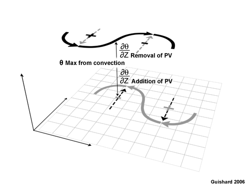
8.3 Tropical Cyclogenesis »
8.3.3.3 Development from an MCS
Mesoscale convective systems (MCS) are organized clusters of convection. Increasing organization of MCS in the 72 h prior to genesis is observed in monsoon region developments and supports the hypothesis of mutual interaction between a mesoscale vortex and large-scale flow.16,46,74 Tropical Cyclone Oliver (1993) provided the first documented case of genesis from the accumulation of mesoscale vorticity.16 Oliver evolved from a cluster of weak mesovortices that merged to become two MCS (Fig. 8.26a and b). Subsequently, one of these MCS developed an eye structure (Fig. 8.26c) and sheared the other system, which became the tropical cyclone rainband (Fig. 8.26d). As these processes were occurring, the low-level relative vorticity of the large-scale monsoon trough was strengthening through diabatic processes. This resulted in a reduction of the Rossby deformation radius (Fig. 8.18) of the broader genesis environment, further concentrating the effects of the convective heating locally.
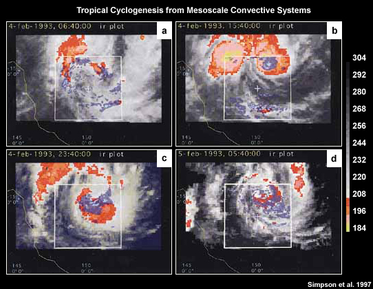
Review the Rossby Radius of Deformation at http://www.meted.ucar.edu/nwp/pcu1/d_adjust/
Realtime microwave satellite data, http://cimss.ssec.wisc.edu/tropic/real-time/tpw/mainTPW.html
8.3 Tropical Cyclogenesis »
8.3.4 Vortex Survival and Evolution
Regardless of how the incipient vortex develops, it must remain coherent until it is in a favorable environment for tropical cyclogenesis to occur and for the storm to intensify. Thus, the response of the mesoscale incipient vortex to environmental forcing will also determine its likelihood of genesis.
An incipient tropical cyclone with weak convection will be more susceptible to weakening even in regions of very low vertical wind shear. The shear will tilt the vortex in the vertical, suppressing vertical motion in the region of the convection, and so weakening the storm.75,76 However, if this vortex experiences only a brief period of vertical wind shear, the vortex can recover from the shear-induced tilt through development of vortex asymmetries.76,77,78 The return of the tropical cyclone to a symmetric storm is sensitive to the radial gradient of storm vorticity.
Strong vertical wind shear [>10‑15 m s‑1 over 850-200 hPa] is often observed to weaken a developing tropical cyclone through suppression of its core convection. However, in some cases, even a weak storm can act to organize itself against the shear, so that it may persist and even intensify in a region of strong vertical wind shear.66,79,80,81 Pre-Hurricane Danny (1997) is one storm that likely benefited from the presence of moderate vertical wind shear (5-11 m s-1 over 850-200 hPa).80 The shear acted to promote convection downshear of Danny, creating additional cyclonic vorticity in that region (Fig. 8.27). This newly formed cyclonic vorticity became organized into a low-level vortex, and then ingested the vorticity associated with the original storm, becoming the primary “Danny” (Fig. 8.27). Increased evaporation due to the strengthening surface vortex enhanced the convection and led to the intensification of Danny into a hurricane.
The case of Danny (1997) suggests that the original thermodynamic environment was unable to support tropical cyclone formation. Although detrimental to the original vortex, shear acted in concert with this vortex to modify the thermodynamic environment (through generation of convection, convergence and moistening of the atmosphere), so that when the Danny vortex reformed, it could intensify (further details of this process are given in Section 8.4.1.2). Thus we see that there is “good shear” and “bad shear” when we think about tropical cyclone development. Whether the shear is either good or bad depends on the intensity and size of storm it encounters, as well as the ocean temperatures and atmospheric moisture.
The case of Danny (1997) suggests that the original thermodynamic environment was unable to support tropical cyclone formation. Although detrimental to the original vortex, shear acted in concert with this vortex to modify the thermodynamic environment (through generation of convection, convergence and moistening of the atmosphere), so that when the Danny vortex reformed, it could intensify (further details of this process are given in Section 8.4.1.2). Thus we see that there is “good shear” and “bad shear” when we think about tropical cyclone development. Whether the shear is either good or bad depends on the intensity and size of storm it encounters, as well as the ocean temperatures and atmospheric moisture.
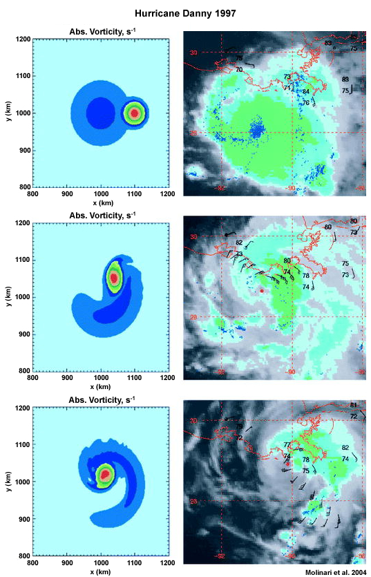
Now let us try forecasting storm development based on our understanding of the impacts of shear and other environmental factors. (Type your response in the box below.)
Given vertical wind shear and SST information for the tropical cyclones shown below, what do you think will happen in the next 36 hours? Make your forecast for each storm:
| a. | The storm intensifies |
| b. | The storm intensity is essentially unchanged |
| c. | The storm weakens |
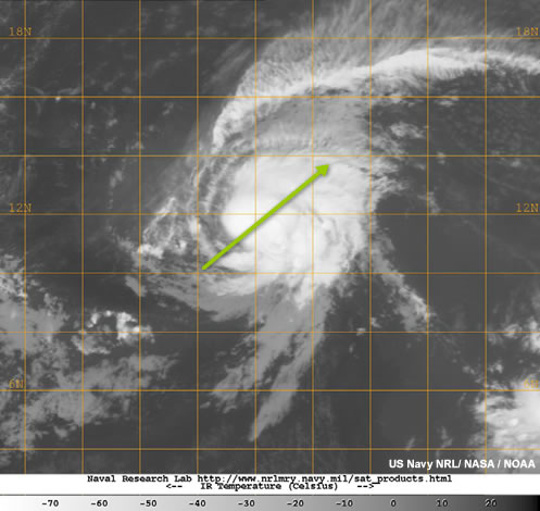 |
Storm 1: SST = 26.5°C Shear magnitude = 15 m s-1/(650 hPa) Shear direction given by arrow |
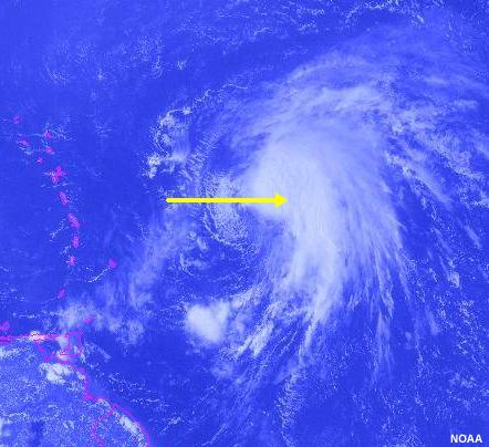 |
Storm 2: SST = 28.0°C Shear magnitude = 10 m s-1/(650 hPa) Shear direction given by arrow |
Feedback:
Using the materials we have covered, you should have been able to devise some simple forecast rules to guide your forecasts of the next stage of development for these two storms. For example:
| (i) | strong vertical wind shear is generally bad; |
| (ii) | vertical wind shear can help the storm intensify if the SST are warm and there are no other negative factors (such as dry air) to slow intensification. |
The correct forecasts for our storms are:
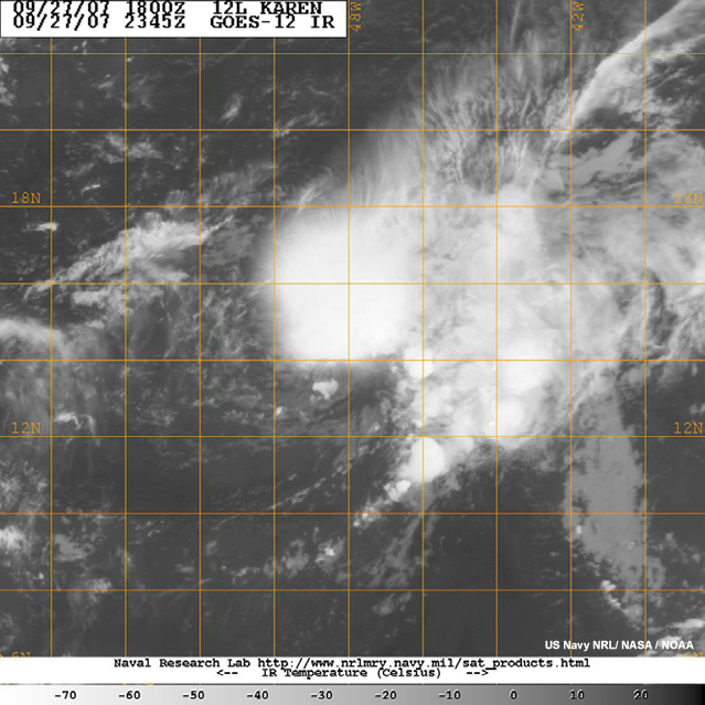 |
|
For Storm 1, the answer is (c) The storm weakens. Why? In this situation the combination of strong shear and cool (for the tropics) SST both acted against intensification. This satellite image is for the same storm 36 hours later. Clearly it is disorganized and has lost most of the active convection around its eye (we see the cirrus shield here). |
| For Storm 2, the answer is (a) The storm intensified. Why? While the shear is weaker than for storm 1, it is still relatively strong. Thus, the warmer SST must have provided a strong enough moisture source so that the storm was able to resist the shear, increase its convection, and intensify. This satellite image is for the same storm 72 hours later. The storm has developed a symmetric structure with a closed eyewall and a clear eye. |
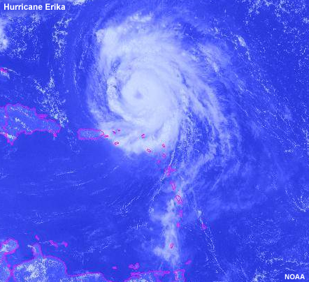 |
As demonstrated with the case of Hurricane Danny just discussed, moist convection can act to reduce the impacts of vertical wind shear. However, as we shall see, all moist convection is not created equal — and convection is not always immediately good for a storm.
The spatial distribution of convection within the vortex can have a large impact on the early evolution of a tropical cyclone.82 Convection developing in a sub-saturated environment will entrain dry air which evaporates the rain in the downdraft, and so delivering cool and dry downdraft air into the boundary layer under the convection. Clearly, this will dry and stabilize the boundary layer locally,70 suppressing further convection (Fig. 8.28). A region with high mid-tropospheric relative humidity supports "good" convection since the moist convective downdrafts in this environment will maintain a moist boundary layer and so will support continued core convection in the developing storm. Should the eyewall convection be cut off, an outer ring of active convection may become established.67,82 This "peripheral" convection spins up the tangential wind and associated radial pressure gradient well outside the radius of maximum winds and reduces the radial pressure gradient closer to the storm center, weakening the low-level inflow to the core. The secondary circulation (in-up-and-out) of the storm now feeds this outer convection, resulting in subsidence in the vicinity of the old eyewall. The subsidence weakens the eyewall convection, suppressing mid-troposphere moisture buildup in the core and weakening the peak surface winds. The peripheral ring of convection is now dominant and modulates the location of subsequent convection.82 Should the original eyewall collapse completely, the ring of peripheral convection may contract to form a new eyewall. Conservation of absolute angular momentum suggests that the storm should eventually reintensify through this process.34,83
Greater lightning activity is often observed in the rainbands and eyewall in weaker tropical storms.37 An example of this is given in Fig. 8.29: even though the magnitude of the vertical wind shear impacting Hurricane Bertha (1996) was almost twice that experienced by Tropical Storm Alberto (1994) as it weakens after landfall, Alberto had dramatically more lightning. This distribution of convection (and associated lightning) is consistent with the development of deep divergent circulations in the storms75 and the greater disruption to the weaker system.
8.3 Tropical Cyclogenesis »
8.3.5 Summary of Possible Tropical Cyclogenesis Mechanisms
In the last 10 to 15 years, a much broader range of pathways to tropical cyclogenesis have been recognized. The most recently identified mechanisms contributing to tropical cyclogenesis in each of the affected ocean basins are given in Fig. 8.30.
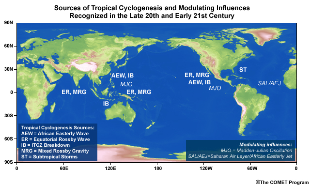
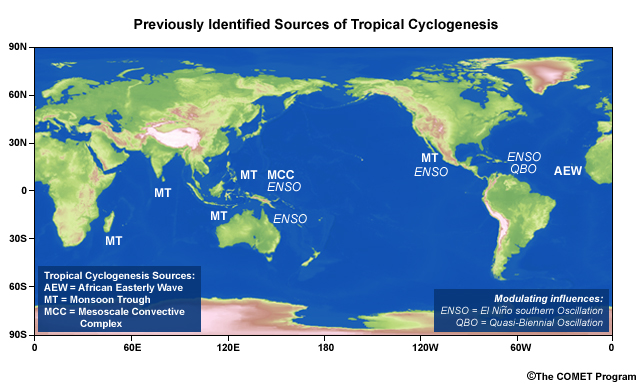
New insights on the large scale impacts on tropical cyclogenesis include clarification of the positive role of shear in the baroclinic development of subtropical precursor disturbances and the basin-wide increase in convective organization through the evolution of the intraseasonal Madden-Julian Oscillation (MJO).84,85
Strengthening of the monsoon trough through active convection and persistence of easterly waves into the western North Pacific have both been demonstrated to increase the likelihood of genesis. In addition, the role of equatorial Rossby and mixed Rossby gravity waves as precursor disturbances for tropical cyclogenesis has been confirmed using satellite observations.
One message comes out of all of these genesis mechanisms: each component of Gray’s genesis parameter41 plays a physical role in preconditioning the environment for genesis, thus modulating storm genesis frequency.
Operational forecasts of tropical cyclogenesis have been developed on two fronts: daily forecast models and seasonal forecasts of tropical cyclone activity, expressed in terms of storm and hurricane numbers or storm days.
Operational forecasts of tropical cyclogenesis have been developed on two fronts: daily forecast models and seasonal forecasts of tropical cyclone activity, expressed in terms of storm and hurricane numbers or storm days.
Operational Tropical Cyclone Forecasting
Learn about operational forecasting of tropical cyclones in Chapter 9, Section 9.5. Hear from tropical cyclone forecasters, in their own words! Find out how they create their forecasts, what inspired them to become forecasters, and how they prepared for their careers (Chapter 9, Focus Section 2).
Learn about operational forecasting of tropical cyclones in Chapter 9, Section 9.5. Hear from tropical cyclone forecasters, in their own words! Find out how they create their forecasts, what inspired them to become forecasters, and how they prepared for their careers (Chapter 9, Focus Section 2).
8.4 Intensity
When a tropical cyclone is bearing down on land, the first question that people ask is "Will it hit me?" followed shortly thereafter by "How intense is it?" Both questions amount to "How will it affect me?"
In this section, we will review (i) the concept of Potential Intensity (PI) and its relationship to actual intensity, (ii) modulation of storm intensity by its environment, (iii) inner core impacts on storm intensity and (iv) satellite estimation of tropical cyclone intensity.
8.4 Intensity »
8.4.1 Potential Intensity (PI)
In 1948, Palmén86 explained the 26-27°C lower SST bound for tropical storm formation in terms of the boundary layer equivalent potential temperature (θe) needed to sustain tropical deep convection. This analysis provides insight into the source of the empirically determined lower bound on SST for tropical cyclogenesis. But how intense can a tropical cyclone become?
Two dominant alternative theories compete to explain the limits on tropical cyclone intensity — its Potential Intensity (PI). PI is the maximum possible surface wind speed or minimum central pressure attainable by an individual storm given the constraints imposed on it by the thermodynamics of its environment. The fundamentals of these two PI theories are reviewed here..
8.4 Intensity »
8.4.1 Potential Intensity (PI) »
8.4.1.1 Early Theories of Potential Intensity: CISK
Banner Miller developed a theoretical model for hurricane intensity in 1958.87 He related the maximum intensity of a tropical cyclone to the (i) SST at the center of the storm, (ii) relative humidity of the surface air in the storm; (iii) lapse rates in the environment of the storm, and (iv) potential temperature at the top of the storm and its height above the surface. He reasoned that the surface temperature and humidity (and thus, to the equivalent potential temperature, θe, of the surface air) determined the temperatures attained aloft in convection—and thus, the potential temperature at the top of the eyewall. Miller calculated the hydrostatic pressure drop due to the potential temperature anomaly associated with the eyewall convection, concluding that subsidence warming in the eye must be included to attain the range of observed minimum central pressures.
Miller's model of the mature hurricane is consistent with Conditional Instability of the Second Kind (CISK), a theory for tropical cyclone maintenance and intensification that was proposed, in the early 1960s, by two groups simultaneously.52,53 According to the "CISK view", the frictional convergence of warm, moist (high θe) boundary layer air into the tropical cyclone determines the amount of latent heat release in the eyewall convection (Fig. 8.31). In this view, boundary layer convergence provides all of the moisture available to ascend into the convection and condense as rain—thus providing the latent heat release that is converted to mechanical energy: the winds of the tropical cyclone. However, friction has two roles in CISK: (1) deceleration of surface winds (below gradient wind balance) is the cause of (2) frictional convergence that imports the moist, boundary layer air. Thus, to intensify the storm, latent heat release must provide mechanical energy in excess of that lost to the frictional deceleration creating the convergence. Hence, if the energy from the latent heat release balances the energy lost to surface friction, the storm will maintain its current intensity. If the mechanical energy due to latent heat release exceeds the energy lost to surface friction, the tropical cyclone will intensify.54
One important component of the CISK theory is that it relies on the existence of an incipient disturbance to create the convergent inflow. Many tropical disturbances exist, but only a few develop into tropical cyclones.42 The success of an individual disturbance depends upon its environment.71,88
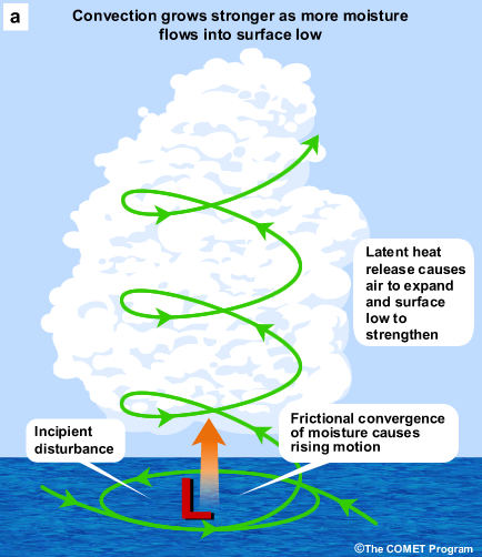
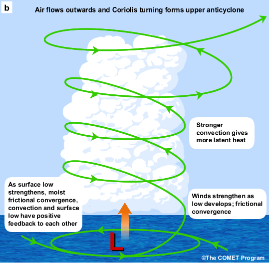
8.4 Intensity »
8.4.1 Potential Intensity (PI) »
8.4.1.2 WISHE: A Carnot Cycle Theory of Potential Intensity
An alternative view of a tropical cyclone is to consider it to be a closed system, a "Carnot engine"89,90 (Fig. 8.32), rather than the moist, frictionally driven convective "chimney" of CISK. A Carnot engineg is a closed system in which heat energy is converted to mechanical energy. As with the CISK theory, this WISHE tropical cyclone intensity theory relies on the presence of a finite amplitude incipient disturbance.14
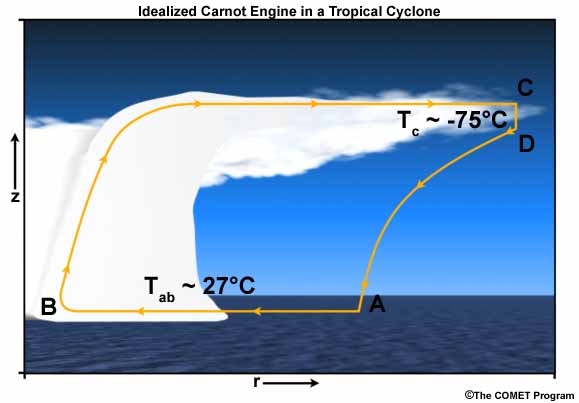
The four “branches” (Fig. 8.32) are: (1) isothermal inflow of near-surface airh (A-B); (2) moist adiabatic ascent in the eyewof the Carnot cycleall convection and outflow just below the tropopause (B-C); and (3) sinking of cooled air in the environment far from the tropical cyclone center (C-D). To close the system, (4) the cooled air is assumed to return to the tropical cyclone environment adiabatically (D-A).
Flow from B to C and D to A is along constant angular momentum surfaces, although
the model assumes that surfaces of angular momentum have constant saturated
equivalent potential temperature ( ) above the boundary layer that is equal to θe of the boundary layer air. Variations of moisture and frictional effects cause these surfaces to diverge in the boundary layer itself.
While the "Carnot cycle tropical cyclone" is drawn as a closed system in the conceptual model (Fig. 8.32), the link between the branch sinking far from the storm center and the boundary layer inflow is not supportable from observations. Tropical cyclones exist in a complex fluid system (the atmosphere) and are not truly isolated systems. Further, a downwards flux of heat through the top of the boundary layer also warms it. This process is absent in all of the PI models described. In spite of its many simplifying assumptions, the Carnot cycle PI theory provides a reasonable estimate of the upper limit for tropical cyclone intensity in a given environment, although not for the actual intensity at any given time.
Let us now consider the first two branches of the Carnot cycle: the inflow and transport of air aloft in the eyewall and outward near the tropopause. Inflow in the atmospheric boundary layer is assumed to be isothermal, even though the air is moistening due to evaporation from the sea surface and the surface pressure is dropping (since the need for an incipient disturbance discussed in Section 8.3 means that air is already flowing towards the center of a low pressure system). This means that heat must be being added to the inflowing air, otherwise the dry adiabatic expansion (due to the surface pressure drop) and evaporative cooling would both decrease the surface air temperature. In the strict formulation of the Carnot model, the heat added to keep the surface air isothermal can come from two sources: sensible heat flux at the ocean surface (warm water heating the air via conduction) and heat release due to the frictional deceleration of the winds as they flow over the ocean surface.
Let us now consider the first two branches of the Carnot cycle: the inflow and transport of air aloft in the eyewall and outward near the tropopause. Inflow in the atmospheric boundary layer is assumed to be isothermal, even though the air is moistening due to evaporation from the sea surface and the surface pressure is dropping (since the need for an incipient disturbance discussed in Section 8.3 means that air is already flowing towards the center of a low pressure system). This means that heat must be being added to the inflowing air, otherwise the dry adiabatic expansion (due to the surface pressure drop) and evaporative cooling would both decrease the surface air temperature. In the strict formulation of the Carnot model, the heat added to keep the surface air isothermal can come from two sources: sensible heat flux at the ocean surface (warm water heating the air via conduction) and heat release due to the frictional deceleration of the winds as they flow over the ocean surface.
Air transported by moist adiabatic ascent from the surface to the top of the eyewall has the same saturation equivalent potential temperature, (an approximation of the moist static energy). As a result, we can calculate the temperature difference between the air at the surface and the top of the tropical cyclone if we know (i) the value of for the boundary layer air directly under the eyewall and (ii) the height of the tropopause (the maximum height of the outflow layer). This gives us the characteristics of the moist adiabatic outflow of the Carnot engine (Fig. 8.32). As we will discuss below, it is this temperature difference between the surface and tropopause that tells us how much energy we can get from the system.
To a good approximation, as the air ascends, it is flowing along constant angular momentum surfaces, so there is an inherent assumption this model that angular momentum surfaces have constant . Angular momentum is calculated from a combination of wind speed and distance from the center of the coordinate system (in this case, the center of the tropical cyclone), and the winds in a tropical cyclone rotate more slowly as we look higher above the surface and as we move to larger radii. This means that surfaces of constant angular momentum must slope outward with height, in agreement with the schematic in Fig. 8.32. This is consistent with the sloping nature of the eyewall evident in the photograph from Hurricane Ivan (2004) (Fig. 8.33).
The reasons for the slope of constant absolute angular momentum surfaces in a tropical cyclone and the link to the eyewall structure are discussed in Box 8–6.
The reasons for the slope of constant absolute angular momentum surfaces in a tropical cyclone and the link to the eyewall structure are discussed in Box 8–6.
We have seen that the source of energy for the theoretical Carnot cycle tropical cyclone is the underlying ocean. Evaporation, sensible heat flux and heat from friction combine to maintain an isothermal and increasingly moist boundary layer inflow to feed the deep convection of the eyewall. In the traditional CISK view of tropical cyclones,52,53,87 frictional convergence of moist boundary layer air provides fuel for latent heat release in the eyewall; this combines with subsidence within the eye to create and maintain the warm core of the tropical cyclone, so lowering the surface pressure. In the Carnot cycle view, the air rises nearly moist adiabatically in the eyewall, conserving while becoming increasingly dry due to rain.70,90 The combination of pressure drop and drying results in much cooler temperatures in the outflow layer (just below the tropopause) than the boundary layer inflow temperatures (which are taken to be the same as the SST) (Fig. 8.32). This temperature difference between the ocean surface and the tropopause provides the thermodynamic energy to drive the system.
We calculate the efficiency, ε, of the tropical cyclone Carnot engine to determine the fraction of the heat energy that can be converted into mechanical energy. Using typical values for the SST and tropopause temperatures (Fig. 8.32), we solve for ε:
 (6)
(6)So we see that approximately one third of the available heat energy can be converted into mechanical energy.
How does this translate to TC winds? Given the drop in the central pressure under the eye (which is solved for in the Carnot cycle model) and assuming a distance to the undisturbed environment and an environmental pressure (model parameters that must be assigned), the gradient wind distribution for the three-dimensional wind field can be calculated.89,90 These calculations provide reasonable wind estimates for observed, very intense tropical cyclones.
Three applications of PI illustrate its utility for understanding the evolution and impacts of real tropical cyclones: (i) inference of maximum possible intensity for an observed tropical cyclone anywhere on the globe (Fig. 8.34) ; (ii) providing a reality check upper bound on SHIPS forecasts of actual storm intensity by comparing them against the PI (see Section 9.5.3); and (iii) studying the "rebound" of the environment back to earlier conditions after a tropical cyclone passage.91
Three applications of PI illustrate its utility for understanding the evolution and impacts of real tropical cyclones: (i) inference of maximum possible intensity for an observed tropical cyclone anywhere on the globe (Fig. 8.34) ; (ii) providing a reality check upper bound on SHIPS forecasts of actual storm intensity by comparing them against the PI (see Section 9.5.3); and (iii) studying the "rebound" of the environment back to earlier conditions after a tropical cyclone passage.91
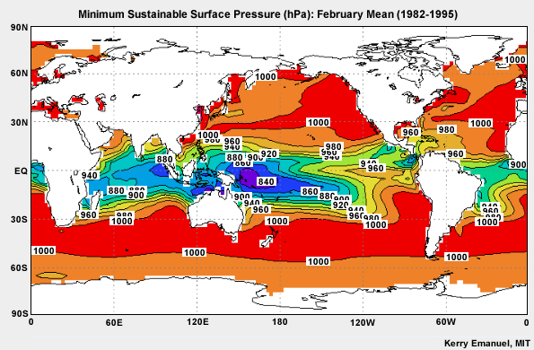
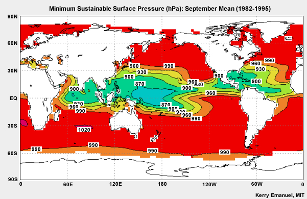
g Our discussion of the Carnot cycle model of a tropical cyclone here will be descriptive. For a more complete, mathematical discussion of this theory, the reader is referred to the source papers.89,90
h Recall that recent analyses13 of the tropical cyclone boundary layer have concluded that it is not isothermal. The impact of this result on this PI model (through changes in the inflow properties) has yet to be tested.
8.4 Intensity »
Box 8-6 Sloping Angular Momentum Surfaces: Linkage to the Eyewall
This section is highly theoretical; experience in dynamic meteorology is recommended.
In meteorology, it is conventional to refer to “specific” quantities.i This is because we do not define individual parcels of the atmosphere and so we are not concerned with the mass or other properties of a parcel, but rather with properties of the atmosphere in general. With this in mind, we will discuss absolute angular momentum, remembering that we are discussing specific absolute angular momentum.
Recall that the (specific) absolute angular momentum,  , is defined as
 , (B8-6.1)
where  is the position vector (relative to the axis) and
  is the absolute velocity of the parcel whose angular momentum is being calculated.
If we are only interested in the azimuthal rotation about the vertical axis, we only need the vertical component of the relative angular momentum:
 , (B8-6.2)
where M is now the magnitude of this vertical component of the absolute angular momentum, r is the scalar radial distance to the location where the rotational wind has speed v, and fo is the value of the Coriolis parameter at the center of the storm. Since  (the rotational wind speed decreases with height),
  , so angular momentum decreases as you go upwards at a constant radius from the center. The contribution of the second term,
  , to the angular momentum gives
  increases as radius increases since fo is constant and r2 increases rapidly with radius. The winds increase, then decrease with radius, so inside the radius of maximum winds and
  is small at large radii (since the decreasing winds and increasing radii oppose).
Combining this information on M(r,z) leads us to outward and upward sloping surfaces of constant absolute angular momentum. Since a fluid will flow along surfaces of constant absolute angular momentum in an adiabatic system, this confirms the near-moist adiabatic nature of this ascent. So now that we agree that (i) the sloping eyewall is a constant angular momentum surface and (ii) for our isolated, symmetric tropical cyclone air flowing along this surface must remain moist adiabatic, let us continue our exploration of the remaining aspects of the Carnot cycle theory.
i "Specific" quantities are quantities that are normalized per unit mass. For example, mass is represented by the inverse density, α, which equates to volume per unit mass.
8.4 Intensity »
8.4.2 Environmental Factors Limiting Tropical Cyclone Intensity
The conditions assumed in the CISK and WISHE conceptual tropical cyclone models—warm ocean waters,86 much cooler outflow temperatures,87 boundary layer convergence, and high relative humidity and accompanying convection52,53 are all present for every tropical storm. So why does every tropical cyclone not intensify to 100 m s-1? Because reality is not the ideal! The large–scale environment changes under the influence of other weather systems.
Variations in the same environmental factors governing intensification can also limit the intensity of a storm: insufficient humidity, cooler SST or warmer tropopause, dry air intrusion, a region of strong baroclinicity are all inhibitors of intensification. "Potential" intensity is only achievable when these factors combine favorably. While these environmental characteristics can inhibit intensification, taking these factors to the other extreme, for example, no vertical wind shear and very warm waters, does not provide the ideal environment for a storm to reach its PI.
The actual intensity of a tropical cyclone that is moving rapidly out of the tropics can even exceed its PI! These storms are most likely undergoing extratropical transition (Section 8.5). Since the environment for this storm is changing so rapidly, its intensity cannot adjust quickly enough to the current environment of the storm so the current intensity tells you more about where the storm has just been than where it is now.
The actual intensity of a tropical cyclone that is moving rapidly out of the tropics can even exceed its PI! These storms are most likely undergoing extratropical transition (Section 8.5). Since the environment for this storm is changing so rapidly, its intensity cannot adjust quickly enough to the current environment of the storm so the current intensity tells you more about where the storm has just been than where it is now.
Figure 8.35 is reproduced from a study92 of the observed distribution between intensity and SST. The 20–year period chosen was predominantly in the satellite era (1967–1986). The SST range plotted is from 15–35°C. All times for all storms in the dataset were included in the analyses depicted in Fig. 8.35, so we should interpret these results in terms of the storm lifecycle.
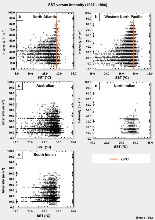
Three conclusions can be drawn from Fig. 8.35:
- Basins without regular reconnaissance flights (panels (c)–(e)) have intensity distributions that emphasize key intensity values (likely reflecting a dependence on satellite-based algorithms to estimate intensity)
- Storm intensity increases dramatically for "tropical" SST> 25°C or so
- The two basins with reconnaissance (panels (a) and (b)) show a uniform distribution of intensity across the observed SST range applicable. This means that stronger storms are restricted to a smaller, warmer range of SST.
What factor(s) might make the warm near-equatorial waters unfavorable for tropical cyclone development? Why might a storm not intensify if it was in an environment with warm SST, no land or dry air, and no vertical shear? Hint #1: the wind speed right at the ground must be very slow. Hint #2: the warm temperatures of the ocean surface do not extend all the way to the bottom of the ocean.
(Type your response in the box below.)
Feedback:
The warm near-equatorial SST are unfavorable for tropical cyclone development since this is also a region of vanishing Coriolis parameter and a region where the sign of cyclonic potential vorticity changes. As a result, it is difficult to create a balanced, cyclonic incipient disturbance to intensify into a tropical cyclone. There are a few exceptions to this where storms form within 5° or so of the equator—for example, Hurricane Ivan (2004). These are usually very small ("midget") cyclones while they are close to the equator.61
See Section 4.1.1.2 for more on this topic.
See Section 4.1.1.2 for more on this topic.
Now why could weak vertical wind shear limit storm intensity? Given the weak environmental winds near the surface, some vertical wind shear is needed to advect the storm along.93,94 Without this environmental advection, a storm will have relatively slow motion. The side–effect of this slow motion over water is that the storm will mix cooler ocean water from below the thermocline. A small contribution to this surface ocean cooling may also come from the storm rainfall. Thus, a storm that stays in the same location will cool the waters below it — and thus limit its own peak intensity.95 The shear inherent in the advection of the storm may delay intensification, but if all other factors are favorable it is possible for the storm to ultimately reach its PI.81
8.4 Intensity »
8.4.3 Links between Inner Core Dynamics, Cyclone Structure and Intensity
As we have discussed, the key to a storm maintaining its current intensity or intensifying further is the maintenance of the deep convection surrounding its core. Maintenance of intensification by the WISHE process (described in Section 8.4.1.2) requires a very moist boundary layer.82 Sub-saturated convective downdrafts will lower the relative humidity (and thus, the moist static energy) of the boundary layer,70 limiting the energy available to the storm. It will take a number of hours for evaporation to recover the boundary layer moisture before intensification can resume. These arguments can readily be extended to understand why dry air intrusions (from dry – even desert – land masses or from the SAL in the case of the Atlantic Ocean) negatively impact intensifying tropical cyclones: the dry tropospheric air weakens the convection, creating sub-saturated downdrafts, which subsequently cools the boundary layer and lowers its relative humidity.
In thinking about why every tropical cyclone does not become a 100 m s-1 behemoth, we argued that a minimum level of vertical wind shear is necessary for a storm to maintain its intensity or to intensify further. While this is true, the strong vertical wind shear that leads a storm to begin recurvature causes the majority of storms to weaken.96,97 This weakening can be understood in terms of the reorganization of the storm in adjusting to this new environment.75,98 The tropical cyclone is a fluid vortex and so it is not separate from its environment: the cyclone and environment are part of one system. Thus, we cannot think of the environment blowing past the storm or blowing it over. The environmental wind shear will cause the storm to reorganize through induced convection on the downshear side of the storm that will initially create an asymmetry. Ultimately the storm will eithereither (i) reintensify as a tropical system, having generated sufficient convection to retain its tropical structure in the sheared environment; or (ii) become extratropical (Section 8.5) and reintensify because of the wind shear; or (iii) decay.
These arguments do not apply uniformly across all tropical cyclone intensities. As we discussed in Section 8.2.3.2, the inertial stability of a tropical cyclone increases with increasing intensity. Since inertial stability is a measure of the resistance of a tropical cyclone to external influences, increasingly intense tropical cyclones should be more resistant to adverse environmental effects. For example, a storm rotating with peak surface windspeeds of 50 m s-1 would be less disrupted by strong vertical wind shear than a storm of 20 m s-1. Equally well, a storm whose strong winds extend further from its center will also be more resilient, since this storm will have large values of inertial stability out to larger radius.99 However, the inertial stability of the tropical cyclone decreases dramatically aloft (Fig. 8.14), so the tropical cyclone is susceptible to upper-tropospheric environmental forcing.
There is one environmental exception to this argument of inertial stability providing the tropical cyclone with increased protection against adverse environmental effects: the SST. Since the ocean surface impacts the tropical cyclone from below, no amount of inertial stability will “protect” the tropical cyclone from adverse impacts due to cool SSTs.
8.4 Intensity »
8.4.4 Estimation of TC Intensity by Remote Sensing
Remote-sensing is the primary method of observing tropical cyclones, which spend most of their lifetime over the ocean, outside of the network of in situ instruments. In addition to estimates of intensity, remotely-sensed observations help scientists to understand the large-scale environment and TC internal instabilities, factors which influence tropical cyclone intensity.100,101,102
Instruments include satellite radiometers (IR, visible, and microwave), precipitation and cloud radars (ground, airborne, and satellite), satellite scatterometers, and synthetic aperture radars (SAR). Figure 8.36 illustrates recent advances in satellite radar and microwave observations of tropical cyclone structure.
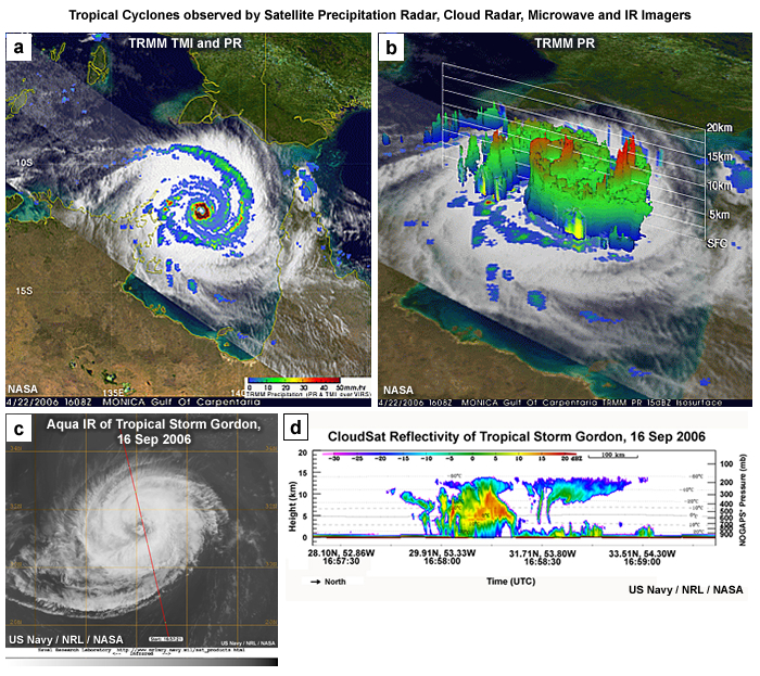
TRMM Radar Animations, http://trmm.gsfc.nasa.gov/publications_dir/multi_resource_tropical.html
US Navy NRL, CloudSat TC images, http://www.nrlmry.navy.mil/tc_pages/tc_home.html
8.4 Intensity »
8.4.4 Estimation of TC Intensity by Remote Sensing »
8.4.4.1 Satellite-IR Estimates
The standard method of estimating TC intensity is by analyzing geostationary longwave (IR) images, except for the North Atlantic and Northeast Pacific, where aircraft reconnaissance flights are routine. With frequently available geostationary IR images (15–30 minutes routinely and 5 minutes in rapid-scan mode), the intensity can be updated for continuous operational forecasting.
In 1975, Vern Dvorak introduced a classification scheme for estimating the intensity of TCs from satellite imagery.103 The “Dvorak Technique”, which was developed using empirical data, relates a numerical index (called the current intensity or CI) to an estimate of the maximum sustained winds (MSW)103 at the surface (Table 8.2).
The Dvorak Enhanced IR technique uses a special enhancement, known as the IR-BD curve, to identify intense convection and changes in the cloud top pattern around the eye. It identifies four basic TC pattern types, the:
|
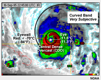
The eye pattern identifies the temperature contrast between the warmest part of the eye and the coldest surrounding convection within 55 km (e.g., Fig. 8.37). The greater the temperature contrast, the stronger the system. The curved band pattern is based on the idea that the more wrapped around the rainbands, the greater the system vorticity. The curved band pattern is often easier to follow in visible images than in IR images. The CDO is the area covered by the cirrus clouds that extend from thunderstorms in the eyewall and rainbands of a TC. The shear pattern examines the distance from the low level center to the CDO, with the principle being that greater involvement of the low level center with the deep convection indicates a stronger system. The CDO appearance is judged on its size and degree of banding.
| CI | MSW (kts) |
MSLP (hPa) |
|
| Atlantic | WestPac | ||
1.0 |
25 |
||
1.5 |
25 |
||
2.0 |
30 |
1009 |
1000 |
2.5 |
35 |
1005 |
997 |
3.0 |
45 |
1000 |
991 |
3.5 |
55 |
994 |
984 |
4.0 |
65 |
987 |
976 |
4.5 |
77 |
979 |
966 |
5.0 |
90 |
970 |
954 |
5.5 |
102 |
960 |
941 |
6.0 |
115 |
948 |
927 |
6.5 |
127 |
935 |
914 |
7.0 |
140 |
921 |
898 |
7.5 |
155 |
906 |
879 |
8.0 |
170 |
890 |
858 |
The following basic steps in the Dvorak Technique are illustrated in a decision tree in Fig. 8.38:
- Find the cloud system center, which is the point towards which the cloud bands spiral. Center location is fairly easy if the low-level circulation is exposed, otherwise, the center is identified by other features such as cirrus outflow, animation, or extrapolation;
- Make two-quasi-independent estimates of the intensity of the TC. Assign a T or "tropical" (T No.), which is related to storm intensity (Fig. 8.39);
- Choose the best estimate;
- Apply selected rules to determine final intensity.
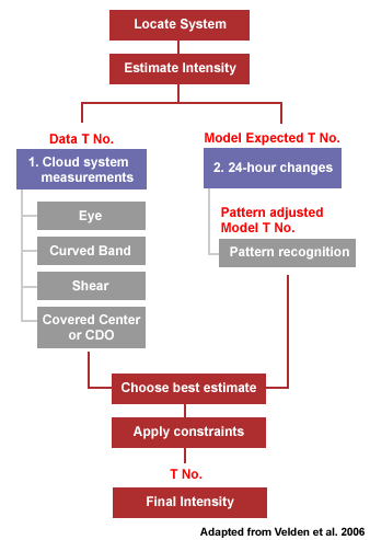
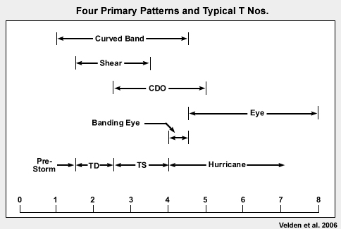
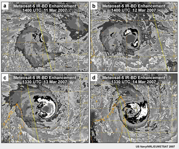
Figure 8.40 shows changes in the cloud organization, central area of the cyclone, and rain bands as Tropical Cyclone Indlala intensified. Between 11 and 12 March, no eye is observed in the IR but the CDO expands and the bands become more curved. During 13 and 14 March, the formation of a small eye (with warmer temperatures relative to the eyewall), the expanded area of very cold cloud in bands around the eye, and a more symmetric cold cloud pattern indicate the increased intensity of Indlala.
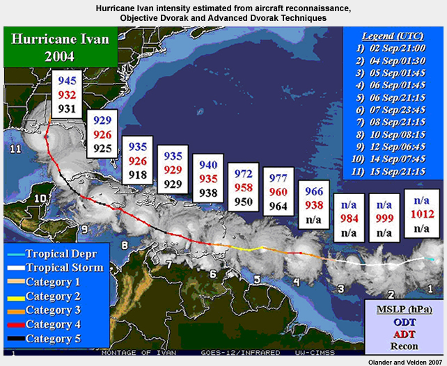
The Dvorak Technique has been updated104 and automated106 through the use of digital IR data and objective algorithms that are based on the original empirical relationships. First was the Objective Dvorak Technique (ODT), then the Advanced Objective Dvorak Technique (AODT), and, as of 2006, the Advanced Dvorak Technique (ADT). An example of comparison between aircraft reconnaissance observations of the intensity of Hurricane Ivan (2004) with both the ODT and ADT is presented in Figure 8.41.
IR analysis is also used to identify annular hurricanes objectively.107 Annular hurricanes have strong and steady intensities and are generally 10–40% larger than normal hurricanes in the Atlantic and East Pacific. On IR images, annular hurricanes are distinctly symmetric and have a large circular eye surrounded by a nearly uniform ring of deep convection and little deep convection outside of that ring.107
http://cimss.ssec.wisc.edu/tropic2/misc/adt/info.html
Tutorial on the use of satellite data to define tropical cyclone structure,
http://severe.worldweather.org/iwtc/pptFile/Topic1/Topic1a/IWTC6-rz.ppt
NOAA Regional and Mesoscale Meteorology Branch (RAMMB) Tropical RAMDIS Online, http://rammb.cira.colostate.edu/ramsdis/online/tropical.asp
8.4 Intensity »
8.4.4 Estimation of TC Intensity by Remote Sensing »
8.4.4.2 Satellite Microwave Observations
Microwave radiometers can detect the internal cyclone structure, such as the location of the eye, because microwave wavelengths are strongly attenuated by hydrometeors (droplets or ice crystals) inside of the eyewall and rainbands. IR techniques, meanwhile, observe only the cloud tops and thick cirrus can hide the underlying TC structure. For example, in Fig. 8.42, it is difficult to identify the eye of Tropical Cyclone Indlala from the IR images (upper panels). However, in the 85 GHz microwave images, the eye is prominent (Fig. 8.42, lower panels), providing a reliable indication of a strengthening tropical cyclone. Moreover, the region of cold cloud to the right of the eye, in the IR image, is not associated with deep convection; it shows up as blue in the microwave image. Unfortunately, microwave instruments fly on low-earth-orbiting (LEO) satellites which observe the same cyclone at most twice per day (Chapter 2, Section 2.1.2.2). Multiple daily views of the same tropical cyclone have become more common as the network of LEO satellites continues to expand. Because they show the internal structure of TCs, microwave images are helping to identify intense cyclones many of which display concentric eyewall structures (e.g., Fig. 8B3.2).83
Microwave radiometers can detect the internal cyclone structure, such as the location of the eye, because microwave wavelengths are strongly attenuated by hydrometeors (droplets or ice crystals) inside of the eyewall and rainbands. IR techniques, meanwhile, observe only the cloud tops and thick cirrus can hide the underlying TC structure. For example, in Fig. 8.42, it is difficult to identify the eye of Tropical Cyclone Indlala from the IR images (upper panels). However, in the 85 GHz microwave images, the eye is prominent (Fig. 8.42, lower panels), providing a reliable indication of a strengthening tropical cyclone. Moreover, the region of cold cloud to the right of the eye, in the IR image, is not associated with deep convection; it shows up as blue in the microwave image. Unfortunately, microwave instruments fly on low-earth-orbiting (LEO) satellites which observe the same cyclone at most twice per day (Chapter 2, Section 2.1.2.2). Multiple daily views of the same tropical cyclone have become more common as the network of LEO satellites continues to expand. Because they show the internal structure of TCs, microwave images are helping to identify intense cyclones many of which display concentric eyewall structures (e.g., Fig. 8B3.2).83
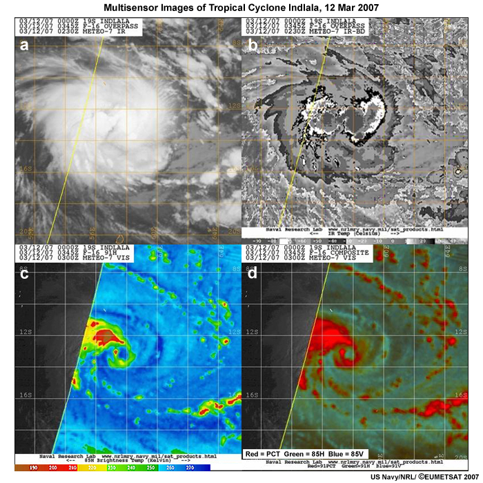
A recent innovation, entitled, The Morphed Integrated Microwave Imagery at CIMSS (MIMIC) developed by Anthony Wimmers and Chris Velden of CIMSS, tries to fill the microwave temporal gap.108
MIMIC creates a sequence of synthetic TC microwave images for the periods between actual satellite microwave observations by four LEO microwave instruments: the DMSP–13/14 SSM/I (85 GHz channel), the TRMM TMI (89 GHz channel) and the Aqua AMSR–E (85 GHz channel). The technique is based on the general expectation that tropical cyclones are roughly axially symmetric in terms of wind speed. The motion of features is the result of interpolation of images, advection, and rotation as the interpolated images are blended. The morphed images are produced every 15 minutes to match the geostationary–IR routine and are available in real-time for five ocean basins. A sample image, for Hurricane Ivan (2004), is shown in Fig. 8.43.
MIMIC creates a sequence of synthetic TC microwave images for the periods between actual satellite microwave observations by four LEO microwave instruments: the DMSP–13/14 SSM/I (85 GHz channel), the TRMM TMI (89 GHz channel) and the Aqua AMSR–E (85 GHz channel). The technique is based on the general expectation that tropical cyclones are roughly axially symmetric in terms of wind speed. The motion of features is the result of interpolation of images, advection, and rotation as the interpolated images are blended. The morphed images are produced every 15 minutes to match the geostationary–IR routine and are available in real-time for five ocean basins. A sample image, for Hurricane Ivan (2004), is shown in Fig. 8.43.
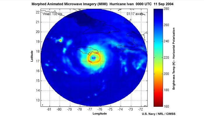
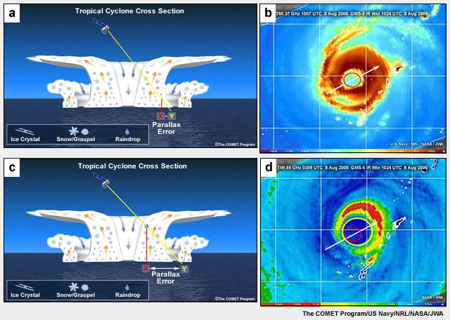
While microwave instruments provide superior TC feature identification, one caveat must be considered in locating the eye of a TC; the effect of parallax. Parallax errors occur when a satellite's slanted viewing angle places features away from their actual location. Figure 8.44 illustrates how parallax errors differ at 85GHz, which is sensitive to ice scattering at high altitudes, and 37 GHz, which is sensitive to emissions from liquid drops at low altitudes. The parallax error is about 5 km at 37 GHz compared with 10–20 km for 85 GHz. The latter frequency has higher resolution (compare Fig. 8.44, b and d) and is the preferred channel for observing tropical cyclone structure and intensity changes.
US Navy NRL Microwave Image Interpretation Training,
http://www.nrlmry.navy.mil/sat_training/tropical_cyclones/ssmi/composite/index.html
8.4 Intensity »
8.4.4 Estimation of TC Intensity by Remote Sensing »
8.4.4.3 Eyewall Replacement Cycles
The concentric eyewall phenomenon or eyewall replacement cycle109 is often observed during periods of intensification or weakening of intense TCs (those with winds greater than 50 m s-1, 115 mph). In general, TC eyewalls contract as they strengthen to the intense TC threshold. After the existing eyewall has contracted to its minimum size for that threshold intensity, the TC enters a weakening phase. All other factors being equal, the TC weakens when an outer eyewall forms; some of the moisture and momentum is taken from the existing eyewall, which dissipates. The outer eyewall contracts gradually and the TC regains its original strength or becomes stronger. For example, major Hurricane Ivan weakened, from a category 5 to a category 4, as it approached Jamaica from the southeast, in part because of an eyewall replacement cycle. Two concentric eyewalls are evident in the radar image from Kingston, Jamaica (Fig. 8.45). The case of Hurricane Georges on 19 September 1998 illustrates the intensification phase of the eyewall replacement cycle. Fig. 8.46 shows TMI images of Hurricane Georges during a period of intensification when the concentric eyewalls were replaced by a single eyewall.
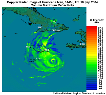
Eyewall replacement cycles can last as short as 12–18 hours to as long as 2–3 days (Figs. 8.45 and 8.46). Some intense TCs undergo multiple eyewall replacement cycles. The West Pacific has the largest percentage of intense storms which exhibit double eyewall structure because many can travel longer distances before encountering land, cool SSTs, or other unfavorable environmental conditions.
New satellite analyses are being developed to objectively identify eyewall replacement cycles. By enhancing the signal to noise ratio of the images, Kossin and colleagues (J. Kossin, personal communication) found that IR imagery does contain information about the onset of eyewall replacement cycles. The IR information, when combined with microwave image data, is being used to create an objective index to calculate the probability of secondary eyewall formation.
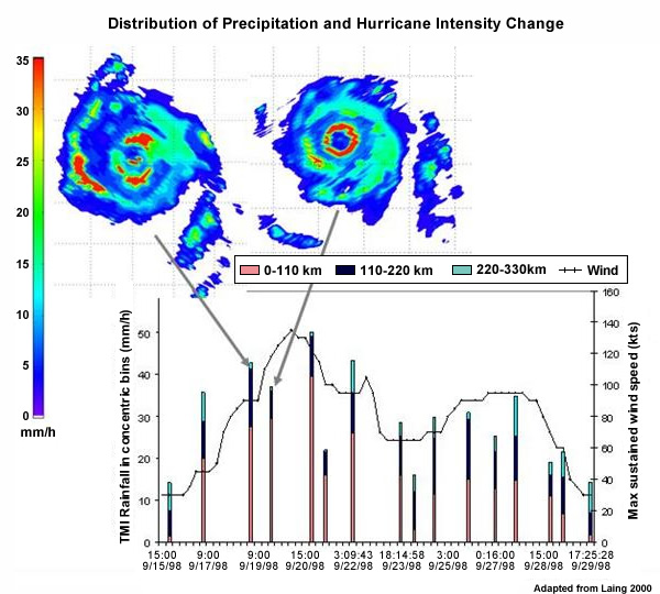
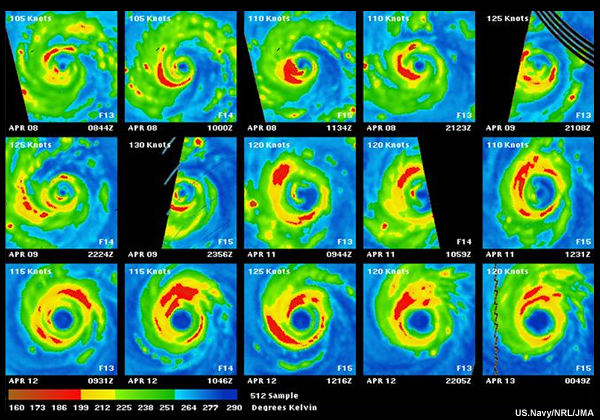
Development of a Secondary Eyewall Formation Index, 60th Interdepartmental Hurricane Conference, http://www.ofcm.gov/ihc06/Presentations/02%20session2%20Observing%20the%20TC/s2-11kossin.pdf
8.4 Intensity »
8.4.4 Estimation of TC Intensity by Remote Sensing »
8.4.4.4 Satellite–derived Winds
It is important to consider TC intensity not only in terms of the central pressure or the radius of maximum winds but in terms of other wind speed radii that are critical to decision makers. The width of evacuation zones is based on thresholds such as the radius of gale force winds (1–minute sustained surface winds between 34 and 47 knots or 17 and 24 m s-1). Wind velocity estimates are also critical to forecasting of storm surge. TC sizes range from Cyclone Tracy (1974), whose radius of gale force winds was only 48 km, to Super Typhoon Tip, which had a gale force wind radius of 1110 km.
Prior to landfall, near surface wind speed and direction are observed by satellite-based microwave scatterometers, which measure the backscatter from small–scale waves on the ocean surface and relate the backscatter to wind velocity. Microwave scatterometers generally perform best in moderate-wind and low-precipitation environments,111 outside of the high–wind and high precipitation region of the eyewall. Microwave sensors such as TMI estimate wind speed away from heavy precipitation regions. Cloud drift winds, although limited by inaccuracies in height assignments, also provide estimates of winds outside of intense convection.104 Figure.8.48 provides examples of satellite–derived winds in and around TCs.
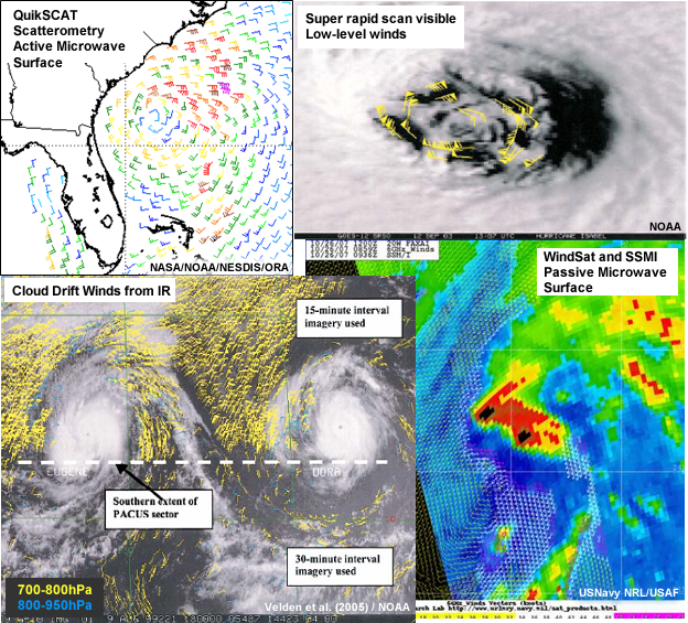
8.4 Intensity »
8.4.4 Estimation of TC Intensity by Remote Sensing »
8.4.4.5 TC Intensity and 34-kt Wind Speed Radius
Statistical relationships between TC intensity estimates from aircraft reconnaissance and satellite IR imagery indicate that the radius of the 34 knot winds could be used to estimate TC intensity. A strong relationship has been found between core intensity and the radius of 34 knot winds.111 Note that relationship between the 34 knot (17 m s-1) wind radii and intensity is not applicable in all situations as the radius of 34 knot winds is also affected by latitude and number of hours since the TC reached tropical storm intensity.112 As TCs move to higher latitudes, they tend to become larger.113
Estimating hurricane wind structure in the absence of aircraft reconnaissance,
http://www.ssec.wisc.edu/~kossin/articles/kossinetal2007WF.pdf
8.4 Intensity »
8.4.4 Estimation of TC Intensity by Remote Sensing »
8.4.4.6 Remote Sensing of Inner Core Dynamical Features
While eyewalls are often observed to be nearly circular, they are occasionally observed to adopt polygonal shapes. Based on theoretical dynamics, numerical simulations, and liquid water experiments114,115,116 the polygonal structures were hypothesized to be associated with mesovortices. Recent observational studies117 show pentagon-shaped reflectivity patterns (Fig. 8.49a, c) associated with mesovortices within the eye (Fig. 8.49c), confirming their existence. These eyewall mesovortices are deep vortex structures in the eyewall convection and so have much smaller horizontal scale than the eye. Wind speed in eyewall vortices can be 10% greater than the rest of the eyewall. Addition of the flows associated with the mesovortices to the flow in the eye results in the polygonal shape observed in the cloud pattern.
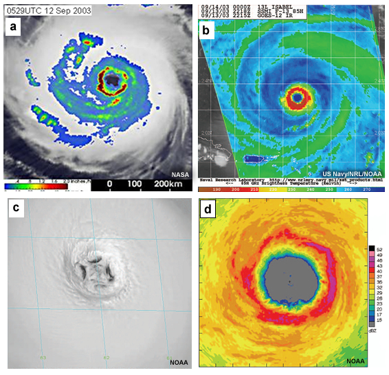
The 2005 Hurricane Rainband and Intensity Change Experiment (RAINEX) made targeted observations in the inner core of Hurricanes Katrina, Rita, and Ophelia in order to understand how changes in their inner core influenced and were influenced by intensity changes. Fig. 8.50 shows a number of interesting features hitherto unobserved, such as filaments of very high reflectivity that are oblique to the concentric eyewall and rainbands. These structures are affected by varying winds as they move around the eyewall and provide clues about how eyewalls transform during rapid changes in intensity. They appear to be similar to structures predicted in theoretical studies and numerical models.113,114,118,119
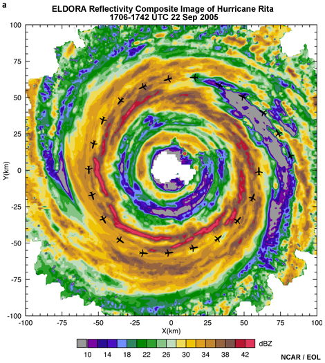
How do these mesovortices affect TC intensity? Theoretical models and evidence in the new observations suggests that the mesovortices contribute cyclonic vorticity which is mixed into the eye. This increase in the local vorticity spins up the eye. In addition, the low-level mesovortices create a secondary circulation that transfers air from the eye to the eyewall and provides additional power to the hurricane heat engine.117 Polygonal eyewalls can also be explained by the vortex asymmetry theory.120,121 Vortex Rossby waves, analogs of the synoptic-scale waves, transport wave energy, momemtum, and heat in the eyewall region. In rapidly intensifying TCs, counter-rotating vortex Rossby waves grow, while straddling the relative vorticity maximum between the eye-wall and the center of rotation. The vortex Rossby waves help to mix high θe air into the eyewall updrafts.
8.5 Extratropical Transition (ET)
Poleward movement of a tropical cyclone is generally expected to lead to the decay of the system as it encounters the hostile, strongly sheared environment and cooler waters (or land) of the midlatitudes. The exceptions to this rule are extratropically transitioning tropical cyclones. The process by which an initially tropical cyclone is transformed into an extratropical cyclone is known as Extratropical Transition (ET – not to be confused with evapotranspiration!). Tropical cyclones typically weaken as they recurve,96,97 but as they move into the extratropics these systems can reintensify into intense midlatitude storms with extensive regions of intense rain and larger gale (and even hurricane) force wind areas than their tropical antecedents.122 The remnant tropical cyclone can also provide a region of enhanced thermal contrast for the later development of an intense midlatitude storm. The rapid forward speed, the large size of their gale force wind area and intense rainfall region, and extraordinarily large ocean waves created by an ET event can persist long after its "tropical storm" status has been discontinued.123
Extratropical cyclones with tropical roots have been tracked poleward of 50°N in the North Atlantic and western North Pacific, with landfalls of initially tropical storms being recorded in western Europe and Alaska (e.g., Fig. 8.1 and Fig. 8.51)! ET systems carry their past with them (evident in their θe and PV signatures)124 and so they transport warm, moist tropical air to high latitudes. This can amplify the midlatitude planetary wave pattern125 and may cause (1) intense midlatitude cyclogenesis even far from the location of the ET event or (2) feed back onto the longwave pattern, modifying interactions between other tropical cyclones and troughs. The impact of this change in the longwave pattern on ET varies: it does not always increase, or decrease, the incidence of ET.126
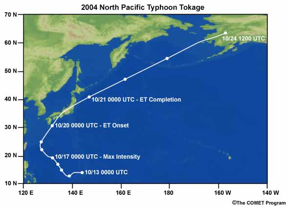
The role of ET in the tropical cyclone climatology has been documented in all tropical cyclone basins. ET studies up until 1960 were limited to only three sets of case studies,127,128,129,130 with increasing interest from the 1950s,3 possibly as a result of Hurricane Hazel's impact on the northeast US and Canada and a spate of typhoon landfalls in Japan. An explosion of research in the 1990s131 has expanded this field of research across all affected basins.
The likelihood of ET for an individual storm depends on (i) the structure and intensity of the tropical cyclone itself, (ii) its thermodynamic environment (convective forcing), (iii) the structure of the midlatitude trough (especially the spatial extent and strength of its associated vertical wind shear) interacting with the tropical cyclone, and (iv) the relative location of the tropical cyclone in the trough.126,132
8.5 Extratropical Transition (ET) »
8.5.1 Global Climatology and Mechanisms Leading to ET
Almost 50% of tropical cyclones making landfall in the North Atlantic undergo ET, with the northeast United States/Canadian Maritimes (1–2 storms per year) and western Europe (once every 10-20 years) being most vulnerable.124 Ten typhoon landfalls in Japan and five in China during 2004 recently emphasized the susceptibility of higher latitude Asian nations to ET (Box 8-9). About 27% of tropical cyclones in the western North Pacific undergo ET;122 for storms in the western South Pacific the statistic is 33%133 and 46% in the North Atlantic.124 However, because the annual tropical storm frequency is much higher in the western North Pacific than the North Atlantic, the western North Pacific basin has the most frequent occurrence of ET events.134 ET is a relatively rare phenomenon in the Indian Ocean, involving only about 10% of tropical storms in the South Indian Ocean.135
Almost 50% of tropical cyclones making landfall in the North Atlantic undergo ET, with the northeast United States/Canadian Maritimes (1–2 storms per year) and western Europe (once every 10-20 years) being most vulnerable.124 Ten typhoon landfalls in Japan and five in China during 2004 recently emphasized the susceptibility of higher latitude Asian nations to ET (Box 8-9). About 27% of tropical cyclones in the western North Pacific undergo ET;122 for storms in the western South Pacific the statistic is 33%133 and 46% in the North Atlantic.124 However, because the annual tropical storm frequency is much higher in the western North Pacific than the North Atlantic, the western North Pacific basin has the most frequent occurrence of ET events.134 ET is a relatively rare phenomenon in the Indian Ocean, involving only about 10% of tropical storms in the South Indian Ocean.135
In each of these basins, the likelihood of ET increases through the storm season, with the peak in ET frequency lagging the peak month for tropical storm activity. For example, in the North Atlantic, the climatological peak of ET incidence is in October, while September is the peak month for tropical cyclone formation.124 Fifty percent of October storms undergo ET; this ratio is 48% in September and below 40% in all other months. ET is mostly likely off the Western Australian coast (the eastern South Indian Ocean) in November, April and May, the monsoon transition months there.135 Finally, there are not strong indications for ET in the western South Indian Ocean off Africa or in the North Indian Ocean.
ET occurs at lower latitudes at the beginning and end of the season, and at higher latitudes during the tropical season peak; these changes in ET location mirror the seasonal movement of the midlatitude jet and the latitudinal extent of the warm SST.
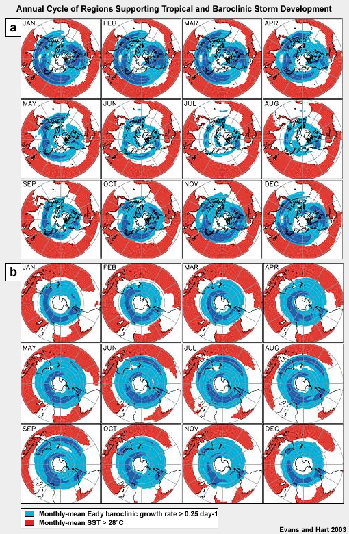
Two diagnostics of the environmental factors leading to ET are depicted in Fig. 8.52: SST > 28°C (favorable for tropical cyclones) and Eady baroclinic growth rate (a proxy for midlatitude cyclone development). The seasonal cycle evident here emphasizes the importance of considering the environment in the region and time of tropical storm activity when deducing likely ET. Based on this analysis (Fig. 8.52), the most favorable situation for a storm to survive through ET is one in which the storm has either strong "tropical" support for development or strong baroclinic development support—or sometimes both.124
The intersection of the monthly tropical cyclone tracks with these diagnostics gives an indication of the likelihood that ET will occur.124 If the mean storm tracks are almost always in one of the development zones, ET is favored in that month. On the other hand, if the mean storm tracks indicate that the storm will traverse a region not indicated as favorable for development (white areas in Fig. 8.52) for any substantial time period, ET is less likely. Finally, only intense tropical cyclones typically complete ET124,136 since they must survive the sheared midlatitude environment until they have completed transition.
The intensity of a tropical cyclone as it begins ET plays a large role in determining whether it will survive transition and ultimately reintensify, or whether it will decay. Genesis location has been related to the likelihood of ET completion.124 Perhaps surprisingly, tropical storms that form at higher latitudes are less likely to undergo ET than storms that form in the deep tropics. This relationship has been linked89 to the intensity of the storms at the time of ET onset. Storms forming in the deep tropics are typically much stronger systems when they commence transition.124
All of these analyses of ET support our earlier statement that the likelihood of ET for an individual storm depends on (i) the structure and intensity of the tropical cyclone, (ii) its thermodynamic environment (represented here by SST), (iii) the structure of the interacting midlatitude trough (represented here by the Eady growth rate), and (iv) the relative location of the tropical cyclone to this trough125,126,132,136,137 (evident through the seasonality of the ET latitude; Fig. 8.52).124
8.5 Extratropical Transition (ET) »
8.5.2 Definitions of ET Onset and Completion
Tropical cyclones are compact weather systems, with relatively symmetric cloud structures and their most intense winds close to the storm center near the surface. Extratropically transitioning tropical cyclones evolve from this structure to become fast moving (>10 m s-1) systems, often resulting in a greatly expanded area of gale force winds. In the process of ET, the peak low-level winds are often much reduced (from the peak tropical intensity) and the maximum winds in the storm now occur aloft. Relative to the storm track, the highly asymmetric storm structure results in strong winds equatorward, and a large expanse of heavy precipitation to the poleward side.122 Thus, to describe the onset and completion of ET comprehensively, measures of both storm symmetry and wind structure must be included—either explicitly or implicitly.
A storm that is commencing the process of ET becomes increasingly asymmetric, due to low–level frontogenesis typically resulting from interaction with a midlatitude trough. This increase in asymmetry is a basic indicator of the onset of transition, but does not guarantee that the system will complete transition28,30,70—many tropical cyclones commence extratropical transition, but decay before completing their evolution into a fully cold-core cyclone.
Storms that remain coherent and become increasingly asymmetric may undergo ET. Completion of the ET process signifies that the tropical system has developed midlatitude storm characteristics, in particular the development of a cold-core thermal wind structure (geostrophic wind speed increasing with height).35,70 Klein et al. (2000)138 add another requirement: that the storm reintensify (in terms of pressure) after completing ET. This last constraint is not applied uniformly. For example, a storm that evolves as described above will be reclassified as "extratropical" by the US National Hurricane Center with no requirement for reintensification. In the context of operational forecasting, it is important to recognize the evolution in the storm structure separately from the evolving intensity because this structure governs the distribution of the significant weather associated with the storm.
A number of new diagnostics have been proposed to characterize ET. Analysis of western North Pacific cases provides guidance on characteristic satellite signatures and environments typical of ET cases29,30 The Cyclone Phase Space (CPS) was demonstrated to be a useful diagnostic of ET for North Atlantic ET cases.36 Composite synoptic environments for ET based on the storm's progression through the CPS agree well with those presented here. The combination of these approaches (satellite and CPS) for diagnosing ET is becoming increasingly widely used in operational centers around the globe. Finally, ET is often poorly forecast by numerical forecast models, providing difficult forecast challenges to the responsible forecast centers. The CPS has been proposed as a metric for evaluating storm structure forecasts.36
Diagnosing and Forecasting ET: Hurricane Michael (2000),
http://www.meted.ucar.edu/norlat/ett/michael/
8.6. Climatology of Tropical Cyclones
Tropical cyclones are a natural part of the climate system (Section 1.2), forming in all tropical ocean basins with the possible exception of the South Atlantic (Fig. 8.1), although rare storms with tropical characteristics are observed in the South Atlantic (Box 8-7). Another location rarely considered as a tropical cyclone center is the Gulf of Oman, so the intrusion of Tropical Cyclone Gonu into this region was an unexpected event (Box 8-8).
Tropical cyclones are a natural part of the climate system (Section 1.2), forming in all tropical ocean basins with the possible exception of the South Atlantic (Fig. 8.1), although rare storms with tropical characteristics are observed in the South Atlantic (Box 8-7). Another location rarely considered as a tropical cyclone center is the Gulf of Oman, so the intrusion of Tropical Cyclone Gonu into this region was an unexpected event (Box 8-8).
8.6. Climatology of Tropical Cyclones »
8.6.1 Seasonality of Tropical Cyclone Formation
Environmental conditions favorable for tropical cyclone formation vary geographically and by season. Broadly speaking, warm ocean temperatures and weak vertical wind shear are two of the necessary, but not sufficient, conditions for tropical cyclogenesis.41
The wind shear tends to be weaker early in the local summer, increasing as the tropical and subtropical oceans warm and the winter Hadley cell strengthens through the local summer and into autumn (Fig. 8.53). Thus, the SH seasonal cycle is out of phase with the NH and generally follows the seasonal monsoon variations (see Section 8.3 for discussion of the large-scale factors governing tropical cyclogenesis).
The wind shear tends to be weaker early in the local summer, increasing as the tropical and subtropical oceans warm and the winter Hadley cell strengthens through the local summer and into autumn (Fig. 8.53). Thus, the SH seasonal cycle is out of phase with the NH and generally follows the seasonal monsoon variations (see Section 8.3 for discussion of the large-scale factors governing tropical cyclogenesis).
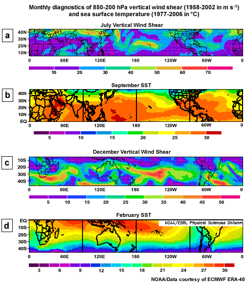
While tropical cyclones are common in most of the global tropics, the western North Pacific is the only basin in which they have been observed in every month of the year (Fig. 8.54). The formation of Tropical Storm Ana in April 2003 and the 2005 Atlantic storms, concluding with Tropical Storm Zeta—for which warnings were issued until 6 January 2006, mean that tropical cyclones have been recorded in the North Atlantic in all months except February and March. Based on long–term statistics of tropical cyclones in the North Atlantic; the "hurricane season" for that basin is defined from 1 June through 30 November. The Eastern North Pacific hurricane season begins on 15 May and also extends to 30 November. In the North Indian Ocean tropical cyclones tend to occur in the monsoon transition months of early (May-June) and late in the wet season (October–November), when the large–scale conditions for genesis are most favorable over that ocean. In the Southern Hemisphere, the tropical cyclone seasons typically extend from November through April, although early and late season storms (October and May) have been observed.
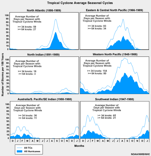
NHC Archive of Hurricane Seasons, http://www.nhc.noaa.gov/pastall.shtml
Japan Meteorological Agency (JMA),
http://www.jma.go.jp/jma/jma-eng/jma-center/rsmc-hp-pub-eg/trackarchives.html
NOAA NWS Climate Prediction Center, Expert Assessments (assessments, advisories, outlooks),
http://www.cpc.ncep.noaa.gov/products/expert_assessment/
http://svs.gsfc.nasa.gov/goto?3354(list of all movies with and without audio)
Video interview with Dr. Jenni Evans, Penn State University Weather World,
http://www.met.psu.edu/research/research-videos
8.6. Climatology of Tropical Cyclones »
Box 8-7 South Atlantic Tropical Cyclone Catarina (2004)
No tropical cyclones have been observed in the South Atlantic since the beginning of the satellite era over 40 years ago – that is, until “Tropical Cyclone Catarina” made landfall in Brazil on 28 March 2004! Because the South Atlantic was thought to be unfavorable for tropical cyclone formation, there was no list of WMO-sanctioned names for this basin. So Catarina was named for the Brazilian state of Santa Catarina where it made landfall. This rarest of tropical cyclones left its mark: at least two people lost their lives, 11 were reported missing and 75 severely injured. Roughly 32,000 homes were damaged and almost 400 were destroyed, giving a total damage estimate of about US $350M.
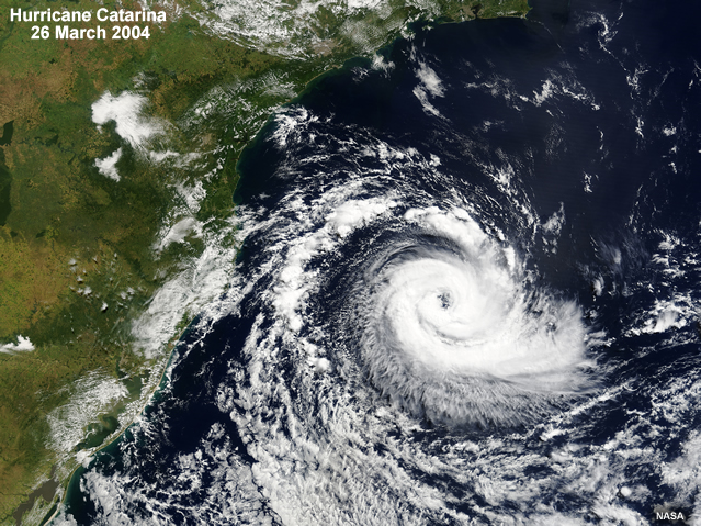
Why was Catarina such a surprise?
Until Catarina, the cooler SST of the tropical South Atlantic and the strong vertical wind shear were thought to preclude tropical cyclone formation. The warmest waters in this region are usually near 26°C (thought to be the minimum SST needed for tropical cyclone formation in the present climate), but Catarina began life as a subtropical storm. In the North Atlantic, subtropical storms form over cooler water and are precursors to tropical cyclogenesis roughly once or twice per season.23
So we see that, storms forming under the right conditions farther from the equator can become tropical cyclones. Intensity theory provides another piece of the puzzle: if the tropopause and surface are cool, it is still possible to achieve hurricane intensity.17 So we see that the formation and intensification of Catarina can be explained by our current understanding of tropical cyclones.
How do we know that Catarina achieved hurricane status (at least 33 m s-1)? The most comprehensive information on Catarina came from the TRMM139 TMI, which sensed the warm core of the system that is typical of a tropical cyclone and the spiral band structure (Fig. 8B7.2), QuikSCAT recorded the surface winds (Fig. 8B7.3).
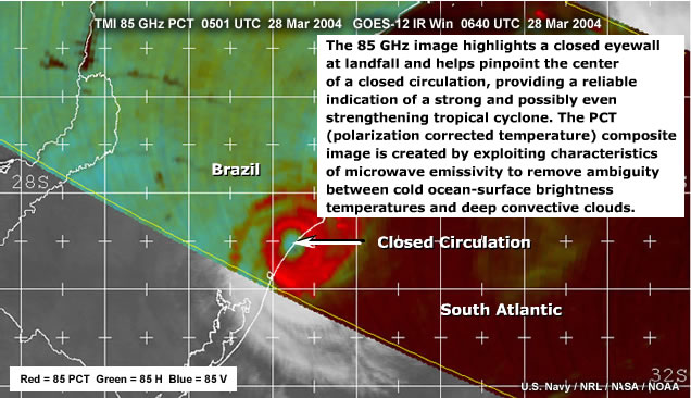
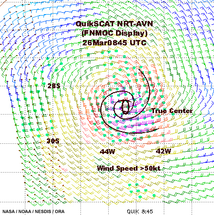
8.6. Climatology of Tropical Cyclones »
Box 8-8 Tropical Cyclone Gonu (2007)
Where in the world would you feel safe from tropical cyclones? How about the deserts of the Middle East? No – even this region can be impacted by tropical cyclones! Tropical Cyclone Gonuj entered the Gulf of Oman as a "Severe Cyclonic Storm" (Box 8–3) with 1–minute maximum sustained winds of 43 m s-1 (83 kts, 153 km h-1, or 95 mph). As the storm moved across the Gulf towards the Iranian coast, it weakened to a tropical storm with winds of around 23 m s-1 (45 kts, 83 km h-1, or 51 mph,) at landfall on 7 June 2007.
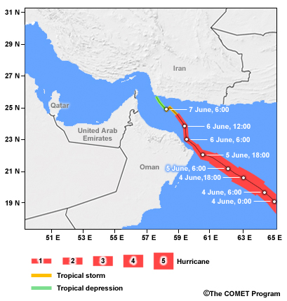
Although Gonu made landfall in Iran, its major effects were in Oman. The Omani capital, Muscat, was impacted by severe winds and associated waves, as well as the torrential rain. Topographic enhancement of the storm rainfall compounded the flooding in Muscat. Gonu was blamed for only three fatalities in Iran; in contrast 25 fatalities were reported in Oman, with about the same number of people reported missing.
j Gonu is the word for a bag made of palm leaves in the Maldives.
8.6. Climatology of Tropical Cyclones »
8.6.2 Intraseasonal Variability
Variation of the necessary conditions for tropical cyclogenesis can lead to clustering of formation events within a storm season. These intraseasonal variations in tropical cyclogenesis frequency are driven by a variety of factors; some, such as the 30–60 day oscillation of tropical rainfall, the MJO,84,85 are tropics-wide phenomena, while others are regional modulators of genesis, such as the Saharan Air Layer (SAL) in the North Atlantic.
Variation of the necessary conditions for tropical cyclogenesis can lead to clustering of formation events within a storm season. These intraseasonal variations in tropical cyclogenesis frequency are driven by a variety of factors; some, such as the 30–60 day oscillation of tropical rainfall, the MJO,84,85 are tropics-wide phenomena, while others are regional modulators of genesis, such as the Saharan Air Layer (SAL) in the North Atlantic.
8.6. Climatology of Tropical Cyclones »
8.6.2 Intraseasonal Variability »
8.6.2.1 Intraseasonal Modulation by the Madden-Julian Oscillation (MJO)
The passage of the “active” phase of the MJO through a region enhances the convective activity locally;140,141 conversely, the “inactive” phase of the MJO suppresses convective activity. Tropical cyclogenesis is likely near the peak of the MJO; Fig. 8.55 shows phases of the MJO and the origins of disturbances that developed into tropical cyclones.
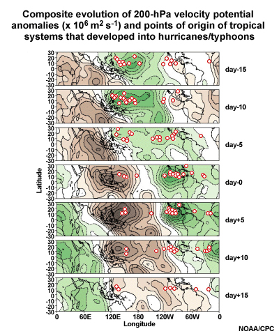
Is the role of the MJO here simply to increase or decrease the likelihood that an incipient disturbance could develop adequate convection to intensify further,50,142,143 or is the question more complex?
(Type your answer in box.)
Feedback:
Different hypotheses have been presented for why and how the MJO modulates tropical cyclogenesis. One perspective is that the increasing convective organization moistens the free troposphere through detrainment of moisture from the clouds. The moisture above the boundary layer provides a favorable environment for sustaining deep convection and for forming larger convective complexes. These organized convective complexes have associated lower tropospheric PV maxima, reducing the local Rossby radius in the presence of convection—one path we have discussed for tropical cyclogenesis144 (Section 8.3.1). An alternative perspective145 is that genesis is more likely for western Pacific storms not because the MJO acts an inherent control on genesis, but rather that the general increase in convective activity in the enhanced phase of the MJO produces many more seed systems from which a tropical storm could develop. However, that hypothesis was contradicted by another study that found that the fraction of systems developing from convective cluster to tropical storm is unchanged between "favorable" [convection active] and "unfavorable" [convection suppressed] phases of the MJO.140 Since the vast majority of tropical cyclones in the Australian region form near the axis of the Australian summer monsoon,15 modulation of this feature by the MJO has been linked to tropical cyclone activity in that region.
Different hypotheses have been presented for why and how the MJO modulates tropical cyclogenesis. One perspective is that the increasing convective organization moistens the free troposphere through detrainment of moisture from the clouds. The moisture above the boundary layer provides a favorable environment for sustaining deep convection and for forming larger convective complexes. These organized convective complexes have associated lower tropospheric PV maxima, reducing the local Rossby radius in the presence of convection—one path we have discussed for tropical cyclogenesis144 (Section 8.3.1). An alternative perspective145 is that genesis is more likely for western Pacific storms not because the MJO acts an inherent control on genesis, but rather that the general increase in convective activity in the enhanced phase of the MJO produces many more seed systems from which a tropical storm could develop. However, that hypothesis was contradicted by another study that found that the fraction of systems developing from convective cluster to tropical storm is unchanged between "favorable" [convection active] and "unfavorable" [convection suppressed] phases of the MJO.140 Since the vast majority of tropical cyclones in the Australian region form near the axis of the Australian summer monsoon,15 modulation of this feature by the MJO has been linked to tropical cyclone activity in that region.
Deep convection in the eastern Pacific has been credited with maintaining the PV gradient reversal63 associated with the off-equatorial movement of Rossby and mixed Rossby-gravity waves into the Pacific confluence zone (Fig. 8.20a). This process is now regarded as a potential source of tropical cyclogenesis (Fig. 8.30a). Maintenance of the dynamic equator by convection highlights the potential importance of convection as a modulator to the dynamic genesis environment, not just a seasonal tracer. Since the MJO is a strong modulator of tropical convection, it has been linked to modulation of the dynamical controls on tropical cyclone genesis too.
MJO modulation of near-equatorial easterly waves over the eastern Pacific affects intraseasonal variations in tropical cyclogenesis in that region.56,143,146 Provided these easterly waves remain coherent in their passage from Africa to the eastern North Pacific, their likelihood of forming tropical cyclones depends on timing rather than initial strength. For cyclogenesis, the easterly wave must interact with the convectively active cycle of the MJO in regions of dynamic instability over the warm tropical waters. As the MJO moves through the region, favorable genesis locations progress eastward and northward, moving with the deep convection in the ITCZ147 The need for all of these complementary factors helps to explain why eastern Pacific cyclogenesis is suppressed in the "unfavorable" phases of the MJO.147
Studies of the easterly wave-MJO system confirmed that barotropic dynamics are an important contributor to coupling the convectively active phase of the MJO with a potential increase in tropical cyclogenesis in the tropical Pacific and Atlantic.148,149,150 The anomalous westerly jet associated with the westerly phase of the MJO is thought to be crucial in the barotropic formation of incipient disturbances across the entire tropical Pacific.
The suggestion is that the convectively active phase of the MJO may create a large scale environment in the eastern North Pacific conducive to tropical cyclogenesis even in the absence of upstream contributors148 (e.g., easterly waves).
Daily monitoring of MJO, NOAA
http://www.cpc.noaa.gov/products/precip/CWlink/daily_mjo_index/mjo_index.html
8.6. Climatology of Tropical Cyclones »
8.6.2 Intraseasonal Variability »
8.6.2.2 Intraseasonal Modulation by the Saharan Air Layer (SAL)
Another large scale modulator of tropical cyclone development in the eastern Atlantic is the Saharan Air Layer (or SAL), first identified in the 1970s.151 From late spring to early autumn the enhanced warm season solar radiation causes deep mixing over the Saharan Desert that results in a dry, well-mixed boundary layer that can extend up to 500 hPa. At its southern end, this Saharan boundary layer air is bounded by the African Easterly Jet, which has peak amplitude of 10–25 m s-1 near 700 hPa (Fig. 8.56). Sand storms created in this dry environment result in suspended particles throughout the layer (Fig. 2.40). Advection of this desert boundary layer over the Atlantic Ocean (often in association with an African easterly wave progression) results in its being undercut by a moist marine layer and creates the SAL. The SAL is thus an elevated layer of very dry, well-mixed air embedded in the Atlantic marine environment (Fig 5.20, Chapter 5).
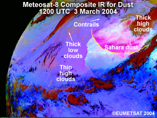
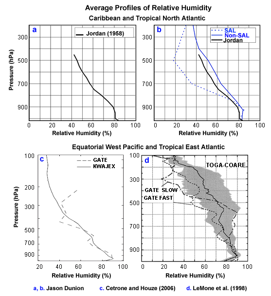
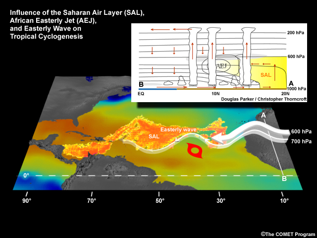
A relationship between the SAL and tropical cyclogenesis is not surprising as the SAL is most prevalent off the West African coast in the Main Development Region (MDR) for Atlantic tropical cyclogenesis.151,154,155 Active convection may persist on its southern and western boundaries, but low relative humidity in the SAL suppresses convection elsewhere. As a SAL outbreak moves off the west coast of Africa, the 700 hPa African easterly jet also elongates offshore due to the meridional temperature gradient between the SAL air and the tropical air to the south.153 Cyclonic shear vorticity south of this mid–level jet accompanied by a mid–level disturbance (the easterly wave) can generate cross–contour flow in the vorticity field, leading to cyclonic vorticity advection and the enhancement of a nearby surface disturbance south of the mid–level easterly jet (Fig. 8.56). Eventual coupling of low– and mid–level disturbances can then lead to tropical depression formation.
This positive relationship between the SAL and tropical cyclone formation is not ubiquitous however. Large SAL outbreaks can weaken any mid–level disturbances in the flow through the generation of a stronger mid–level easterly jet, which causes a more zonally oriented mid–level flow, thus eliminating this tropical cyclogenesis mechanism. In some cases, the SAL can weaken or limit intensification, e.g., Erin in 2001 (Fig. 2.41). As expected then, over–forecasting of genesis by North Atlantic operational numerical models has been attributed to inadequate characterization of the SAL elevated dry layer and accompanying jet.156 Since the early 2000s, a special satellite retrieval algorithm152 (Chapter 2, Section 2.8) and targeted field measurements have increased our knowledge of the structure of the SAL and its role as a modulator of tropical cyclogenesis157 Fig.2.41.
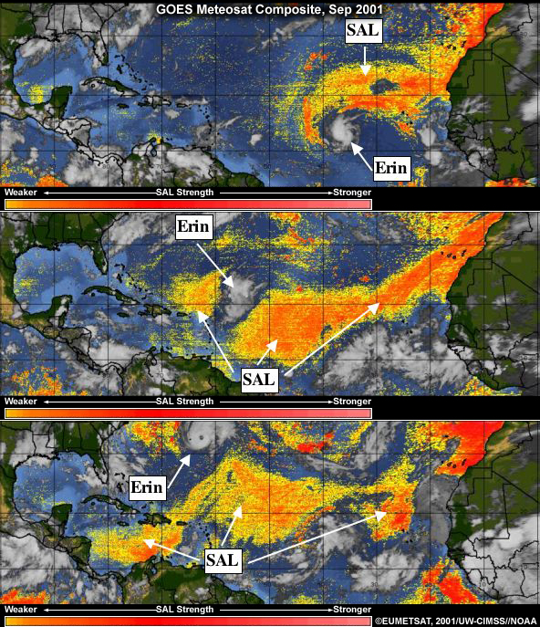
This positive relationship between the SAL and tropical cyclone formation is not ubiquitous however. Large SAL outbreaks can weaken any mid–level disturbances in the flow through the generation of a stronger mid–level easterly jet, which causes a more zonally oriented mid–level flow, thus eliminating this tropical cyclogenesis mechanism. In some cases, the SAL can weaken or limit intensification, e.g., Erin in 2001 (Fig. 2.41). As expected then, over–forecasting of genesis by North Atlantic operational numerical models has been attributed to inadequate characterization of the SAL elevated dry layer and accompanying jet.156 Since the early 2000s, a special satellite retrieval algorithm152 (Chapter 2, Section 2.8) and targeted field measurements have increased our knowledge of the structure of the SAL and its role as a modulator of tropical cyclogenesis157 Fig.2.41.
While the SAL may inhibit development of African easterly waves into tropical storms,152 the waves have been proposed as transportation for Saharan dust158 and so may be implicated in their own demise! Western Sahel rainfall has also been linked to North Atlantic tropical cyclone activity.31,159 Whether the SAL is involved in any intraseasonal modulation of Atlantic storm activity related to western Sahel rainfall—or whether Sahel rainfall is a straightforward proxy for easterly wave genesis frequency—remains an open question.
http://tropic.ssec.wisc.edu/misc/sal/info.sal.m8g10split.html
NOAA Hurricane Research Division SAL project,
http://www.aoml.noaa.gov/hrd/project2007/sal.html
Real-time diagnostics of the SAL,
http://tropic.ssec.wisc.edu/real-time/salmain.php?&prod=splitEW&time=
8.6. Climatology of Tropical Cyclones »
8.6.3 Interannual Variability
Before discussing interannual variability, it is important to understand the difference between annual cyclone activity (frequency and intensity) and the severity of cyclone impacts (landfall frequency, fatalities, and damage). For example, the 2004 western North Pacific and Atlantic tropical storm seasons were not exceptionally active seasons. Yet, Japan suffered a total of ten landfalls and the US state of Florida had three landfalls and suffered the effects of a fourth storm that made landfall in the adjacent state of Alabama (Box 8–9). Furthermore, Hurricane Andrew (1992), a Category 5 hurricane, made landfall near Miami during an inactive season. Thus, commonly–used activity parameters are not necessarily good indicators of impacts, which can be influenced by other, less well-defined, modulators of tropical cyclogenesis and track. For instance, one potential explanation for the impact of the 2004 North Atlantic season is that the large-scale steering flow and equatorial trough160 allowed storms to develop at low latitudes in the eastern Atlantic and to track westward, while remaining unusually close to the equator, before curving poleward as they approached or entered the Gulf of Mexico.
Before discussing interannual variability, it is important to understand the difference between annual cyclone activity (frequency and intensity) and the severity of cyclone impacts (landfall frequency, fatalities, and damage). For example, the 2004 western North Pacific and Atlantic tropical storm seasons were not exceptionally active seasons. Yet, Japan suffered a total of ten landfalls and the US state of Florida had three landfalls and suffered the effects of a fourth storm that made landfall in the adjacent state of Alabama (Box 8–9). Furthermore, Hurricane Andrew (1992), a Category 5 hurricane, made landfall near Miami during an inactive season. Thus, commonly–used activity parameters are not necessarily good indicators of impacts, which can be influenced by other, less well-defined, modulators of tropical cyclogenesis and track. For instance, one potential explanation for the impact of the 2004 North Atlantic season is that the large-scale steering flow and equatorial trough160 allowed storms to develop at low latitudes in the eastern Atlantic and to track westward, while remaining unusually close to the equator, before curving poleward as they approached or entered the Gulf of Mexico.
On interannual timescales, tropical cyclone variability can stem from global patterns of atmosphere or atmosphere–ocean variation, such as the El Niño Southern Oscillation (ENSO)92,161,162 or the Quasi-Biennial Oscillation (QBO)162,163,164,165 of the lower stratospheric wind. Rainfall in the western Sahel has also been associated with variations in the seasonal frequency and intensity of Atlantic tropical cyclones.166,167
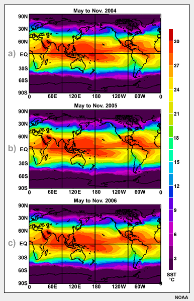
The active 2005 season in the North Atlantic was attributed to extraordinarily warm ocean temperatures in that basin,168,169 however the Atlantic and Gulf of Mexico were similarly warm in 2006 (Fig. 8.57), which was an average year for tropical cyclone activity. Further, the patterns of Atlantic SST in 2004 and 2006 were very similar (Fig. 8.57a,c), yet 2004 was a relatively active year with 15 named storms (9 hurricanes).
Increased understanding of interannual modulators of tropical cyclone activity has inspired seasonal forecasts of likely season severity.161,170,171,172,173 While these forecasts have skill they have largely failed to identify shifts in activity that may be associated with multidecadal variability or, possibly, with global climate change.160,174 To provide context for such shifts in tropical cyclone activity, longer term records of these storms175 and variations in environmental factors modulating genesis176 are necessary. Conventional observational methods cannot provide such records. Thus, proxy records are the mechanism that provide a window on tropical cyclone activity in the distant past. Tropical cyclone variations on decadal timescales are discussed in Section 8.6.4, and Section 4.3.2).
Increased understanding of interannual modulators of tropical cyclone activity has inspired seasonal forecasts of likely season severity.161,170,171,172,173 While these forecasts have skill they have largely failed to identify shifts in activity that may be associated with multidecadal variability or, possibly, with global climate change.160,174 To provide context for such shifts in tropical cyclone activity, longer term records of these storms175 and variations in environmental factors modulating genesis176 are necessary. Conventional observational methods cannot provide such records. Thus, proxy records are the mechanism that provide a window on tropical cyclone activity in the distant past. Tropical cyclone variations on decadal timescales are discussed in Section 8.6.4, and Section 4.3.2).
Japan Meteorological Agency (JMA),
http://www.jma.go.jp/jma/jma-eng/jma-center/rsmc-hp-pub-eg/trackarchives.html
Joint Typhoon Warning Center (JTWC),
http://www.usno.navy.mil/JTWC/annual-tropical-cyclone-reports
NHC Archive of Hurricane Seasons,
http://www.nhc.noaa.gov/pastall.shtml
NHC 2004 Atlantic Tropical Cyclone Reports,
http://www.nhc.noaa.gov/2004atlan.shtml
ENSO monitoring: Real-time data,
http://www.pmel.noaa.gov/tao/jsdisplay/
8.6. Climatology of Tropical Cyclones »
8.6.3 Interannual Variability »
8.6.3.1 Interannual Modulation Due to the El Niño Southern Oscillation (ENSO)
Variation in basin-scale annual tropical cyclone activity can derive from a range of spatial and temporal forcings.41,161,162 ENSO is one of the dominant, multi-year influences on tropical cyclone activity.
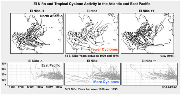
The large-scale atmospheric and oceanic changes accompanying a warm event (El Niño) or a cold event (La Niña) result in shifts in the tropical regions most favorable to tropical cyclogenesis (e.g., Fig. 8.58). For example, the suppression of convection in the Maritime Continent, and extension of the deep convective zone into the central Pacific and Indian Ocean basins during a warm event, is accompanied by changes to the vertical wind shear and SST patterns across the tropics. The result is cooler SST and stronger vertical wind shear in the tropical western Pacific and Atlantic basins as well as warmer SST and weakened vertical wind shear in the central Pacific, eastern North Pacific and the central Indian Oceans. Consequently, tropical cyclone activity in the central Pacific, eastern North Pacific and the central Indian Oceans is generally enhanced during a warm event and tropical cyclones are less prevalent in the central ocean basins in neutral or cold event years. The inverse is true for the western Pacific and North Atlantic Oceans: cold events are more favorable for tropical cyclogenesis and so are typically accompanied by more active tropical cyclone seasons than neutral or warm event years.161,162,167,173
Caution should be used when considering interannual variability and ENSO. Although 1992 was a warm event year (part of a multi–year sustained warm event), it was the year that a Category 5 hurricane made landfall in Miami, Florida. Hurricane Andrew was the first storm—and a very late start—of a relatively quiet season, yet it was the most devastating storm to hit the US mainland in almost twenty years. This demonstrates that links between seasonal activity and landfall frequency, storm intensity, or storm impacts are tenuous.
8.6. Climatology of Tropical Cyclones »
8.6.3 Interannual Variability »
8.6.3.2 Interannual Modulation by the Quasi Biennial Oscillation (QBO)
Another multi-year modulator of interannual tropical cyclone activity is the Quasi Biennial Oscillation of the stratospheric zonal wind (Fig. 8.59, Chapter 4).162,163,164,165 As with ENSO, the effects of the QBO on tropical cyclone activity are regionally dependent.
Another multi-year modulator of interannual tropical cyclone activity is the Quasi Biennial Oscillation of the stratospheric zonal wind (Fig. 8.59, Chapter 4).162,163,164,165 As with ENSO, the effects of the QBO on tropical cyclone activity are regionally dependent.
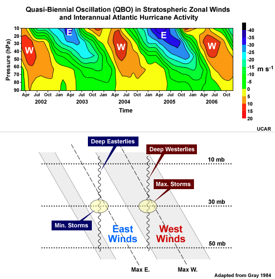
The link between the phasing of the QBO and tropical cyclone activity in the western North Pacific and North Atlantic Oceans161,171,177 lies in the associated changes in the local vertical wind shear. The phases of the QBO tied to more (less) active hurricane seasons result in decreased (increased) vertical wind shear in the lower stratosphere. In the western North Pacific this decrease (increase) in vertical wind shear occurs in the easterly (westerly) phase of the QBO and is linked to enhanced (suppressed) seasonal tropical cyclone activity.164 A westerly QBO (westerly anomaly in the equatorial zonal wind at 30 hPa) during Atlantic hurricane season typically results in a more active season than normal; in contrast, an easterly QBO suppresses seasonal activity with similar effectiveness to a warm event.
8.6. Climatology of Tropical Cyclones »
8.6.4 Decadal Cycles and Long Term Climate Influences
While very long-time (multi–century) changes in the tropical climate have been investigated for decades, tropical cyclone variability on timescales longer than a few years has only recently been recognized.178,179,180,181 Variations in the ENSO phenomenon on decadal timescales have been analyzed from surface pressure and SST records extending back to the mid-19th century or even earlier.182,183 These data have been recovered from observation archives such as ship logs184 or from proxy records.175 These ENSO variations have been proposed to impact typhoon and tropical cyclone activity in the Pacific, and possibly Indian Ocean basins. Long–term records of tropical cyclone activity–such as the six century landfall record for China181–may be used to test this link.
Three possible physical mechanisms have been proposed to explain decadal modulation of ENSO: (i) a coupled internal oscillator in the equatorial Pacific;185 (ii) tropical forcing from midlatitude variability;185 or (iii) slowing of the global meridional overturning circulation leading to decadal SST fluctuations in the Pacific.186 It is not yet clear whether one of these mechanisms or a different mechanism not yet considered will explain this phenomenon.33,34
The third proposed mechanism for interdecadal variability of ENSO builds upon the concept of the Ocean Conveyor Belt or global thermohaline circulation which links the global ocean currents (see Fig. 3.21a).187 The surface ocean currents are driven by formation of "deep water" which sinks deep into the ocean in the northern Atlantic and in the Southern Ocean (Fig. 3.21b).
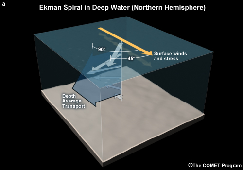
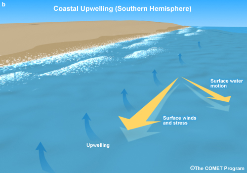
The correspondence between monsoonal rains (drought) over the Sahel region of West Africa, circulation changes in the tropical Atlantic188 and enhanced (reduced) incidence of intense Atlantic hurricanes159,166,189 provides evidence of the link between African easterly wave activity and intense hurricane activity in the basin on multidecadal timescales. Variations in the number of easterly waves are only weakly related to the total number of North Atlantic tropical cyclones in a season. Rather, fluctuations in easterly wave activity contribute to variations in the frequency of intense hurricanes (peak winds in excess of 50 m s-1, corresponding to Saffir–Simpson Cat 3–5).190 This reflects the longer passage over warm ocean waters typical of storms reaching such intensities.
Multidecadal variations in Atlantic hurricane activity have been associated with long-term changes in the ocean temperatures and vertical shear of the horizontal winds in that ocean basin.180 These coupled variations have been termed the Atlantic Multidecadal Oscillation (AMO)Atlantic Multidecadal Oscillation (AMO), which has also been linked to decadal-scale variations in the Ocean Conveyor Belt. If the Ocean Conveyor Belt is accelerated, the tropical Atlantic is warmer than climatology and hurricanes activity increases. By this theory, warm (cool) phases of the tropical Atlantic correspond to transport of waters through the global ocean currents that is faster (slower) than climatology.
Since ocean temperatures and vertical wind shear have been strongly tied to the likelihood of tropical cyclogenesis, the link between these environmental fields and hurricane variability should be unsurprising. The periodic cycling of the ocean conveyor belt187 has been tied to long-term variations in Atlantic Ocean temperatures and extended West African droughts,191,192 apparently making a good case for multidecadal fluctuations in the ocean currents as the source of ocean surface temperature changes, the resultant variations in West African monsoon rainfall and, by implication, easterly wave frequency. It would seem that the case is closed – but science is rarely that straightforward!
Recent work has cast doubt on the multidecadal modulating influence of the oceans on Atlantic hurricanes, opting for an alternative explanation for the 20th Century ocean warming. In this scenario, global climate change combined with the cooling then warming due to the temporal variation in sulfate aerosols through the course of the 20th Century governed the evolution of Atlantic Ocean temperatures.193 This global change (non–AMO) interpretation of Atlantic SST variations raises such fundamental questions as "What is the role of tropical cyclones in the climate?" and "What are the mechanisms through which variations in the base state of the climate affect tropical cyclones?" and "Could changes in tropical cyclone characteristics feedback and influence the evolution of the base state of the climate?"
Theories for the influence of global warming have proposed increases in tropical cyclone intensities linked to the expected continued warming. Newly created datasets112,194 can be used to test these theories and may perhaps provide some insight into the dominant forcing of multidecadal tropical cyclone variations. In the meantime, the tropical cyclone community has prepared a consensus statement on the current understanding of global warming. This statement should be expected to be revised as the science evolves.
WMO statement (long version)
http://www.wmo.int/pages/prog/arep/tmrp/documents/iwtc_statement.pdf
WMO statement executive summary
http://www.wmo.int/pages/prog/arep/tmrp/documents/iwtc_summary.pdf
AMS endorsement of this WMO statement http://www.ametsoc.org/POLICY/wmo.html
8.6. Climatology of Tropical Cyclones »
8.6.5 Seasonal Forecasting of Tropical Cyclone Activity
The first systematic, statistically-based seasonal forecasting methodology for tropical cyclone activity dates back to the late 1970s172 and focused on the Australian region. It was not until 1984 that scientists from Colorado State University began publishing regular forecasts of annual tropical cyclone activity for the North Atlantic basin.162,170
| Group | Basins | Type | Website |
| City University of Hong Kong, China (City U) | Western North Pacific | Statistical | http://aposf02.cityu.edu.hk |
| Colorado State University, USA (CSU) | Atlantic | Statistical | http://hurricane.atmos.colostate.edu |
| Cuban Meteorological Institute (INSMET) | Atlantic | Statistical | http://www.insmet.cu |
| European Centre for Medium-Range Weather Forecasts (ECMWF) | All basins | Dynamical | http://www.ecmwf.int (collaborating agencies only) |
| International Research Institute for Climate and Society (IRI) | All except Indian Ocean | Dynamical | http://iri.columbia.edu/forecast/tc_fcst/ |
| Macquarie University, Australia | Australia/Southwest Pacific | Statistical | http://www.iges.org/ellfb/past.html |
| National Meteorological Service, México (SMN) | Eastern North Pacific | Statistical | http://smn.cna.gob.mx |
| National Climate Centre, China | Western North Pacific | Statistical | http://bcc.cma.gov.cn |
| NOAA Hurricane Outlooks | Atlantic Eastern North Pacific Central North Pacific |
Statistical | http://www.cpc.noaa.gov/index.php http://www.cpc.noaa.gov/index.php http://www.prh.noaa.gov/hnl/cphc/ |
| Tropical Storm Risk (TSR) | Atlantic Western North Pacific Australian region |
Statistical | http://www.tropicalstormrisk.com/ |
Early statistical predictions of North Atlantic seasonal hurricane activity relied predominantly on the phases of ENSO (either prior to the season or predicted for the peak of the season) and the QBO, as well as Caribbean sea level pressures. For example, more tropical cyclones are predicted for cool events (anti–ENSO), west phase of the QBO162 or below–normal Caribbean basin sea level pressures196–and especially if all three coincide. These relationships with seasonal tropical cyclone activity (defined by any of total number of named storms, named storm days, hurricanes or hurricane days) were explained in terms of changes in the tropical Atlantic atmosphere and ocean circulations that modified the necessary conditions for tropical cyclogenesis (Section 8.3.1).
Early statistical predictions of North Atlantic seasonal hurricane activity relied predominantly on the phases of ENSO (either prior to the season or predicted for the peak of the season) and the QBO, as well as Caribbean sea level pressures. For example, more tropical cyclones are predicted for cool events (anti–ENSO), west phase of the QBO162 or below–normal Caribbean basin sea level pressures196—and especially if all three coincide. These relationships with seasonal tropical cyclone activity (defined by any of total number of named storms, named storm days, hurricanes or hurricane days) were explained in terms of changes in the tropical Atlantic atmosphere and ocean circulations that modified the necessary conditions for tropical cyclogenesis (Section 8.3.1).
A variety of statistical models to predict basin–scale tropical cyclone activity around the globe are now available (Table 8.3). Interestingly, even groups forecasting for the same basin use different predictors for the same predictand. For example, while QBO is used as a predictor in the Cuban Meteorological Institute forecasts for North Atlantic hurricane activity,197 it is not included in either the CSU or NOAA models.180,198
A recent innovation in seasonal tropical cyclone forecasting is dynamically-based forecasts.199 In this approach, global forecast models are run out for the season and the number of tropical cyclone-like vortices predicted in these models is counted. Various storm characteristics can be recorded for these modeled storms and predictions can also be issued on these quantities. One example is the accumulated cyclone energy (ACE), a measure of wind energy that is defined as the sum of the squares of the maximum sustained surface wind speed (knots) measured every six hours for all named systems while they are at least tropical storm strength.
A seasonal forecast model must demonstrate skill against a "no skill" baseline prediction to be useful.200 The most common no skill forecast used for operational weather forecast models is a combination of climatology and persistence (known as CLIPER). Evaluations of a number of available statistical seasonal forecast models demonstrated that these had skill against this CLIPER benchmark.195,201 This means that these models have useful information on the likelihood of more or less activity in the upcoming season.
8.6. Climatology of Tropical Cyclones »
Box 8-9 Unusual Tropical Cyclone Seasons around the Globe
Every so often a tropical cyclone season will catch the attention of even the most disinterested observers of the tropics. The maps that follow here depict a selection of recent seasons that have caught the imagination of many across the globe.
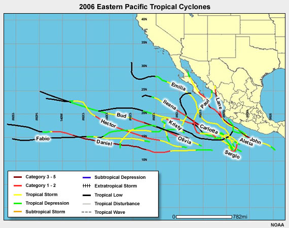
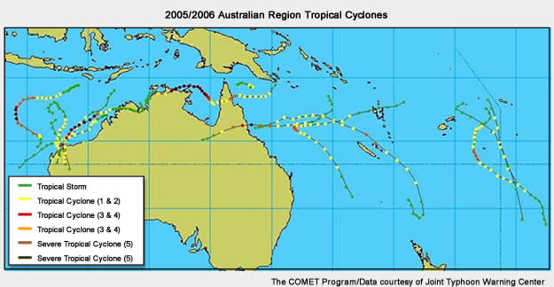
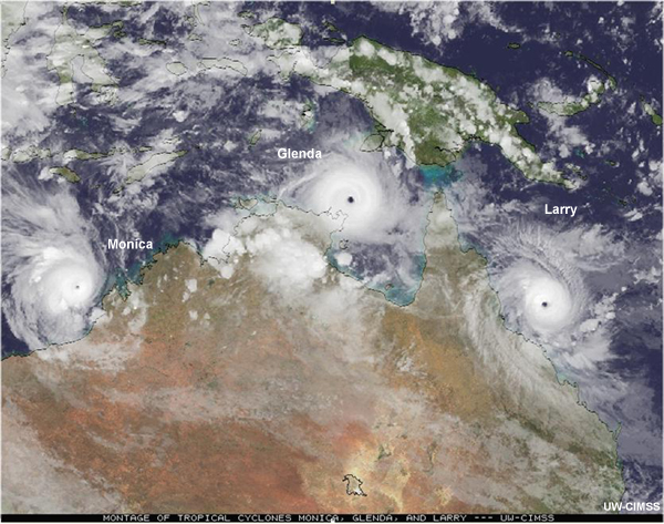
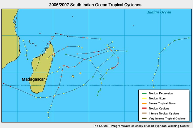
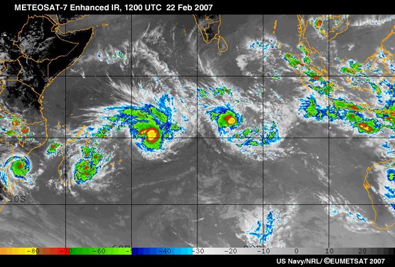
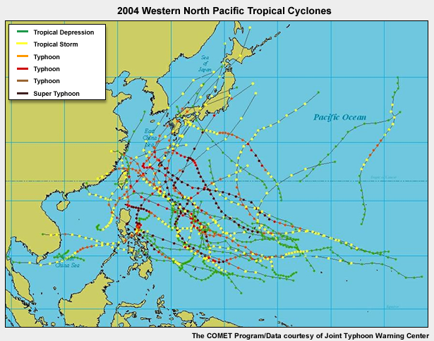
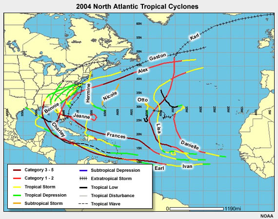
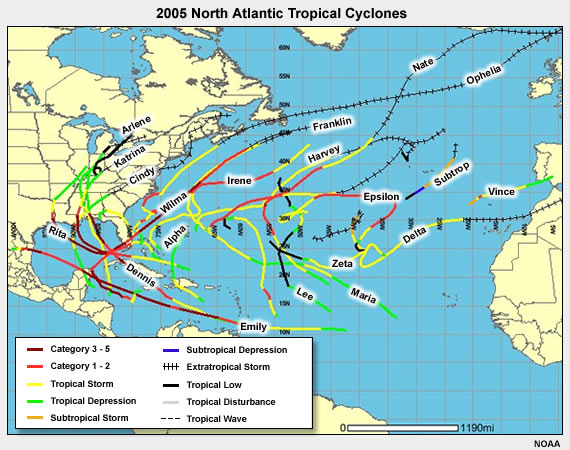
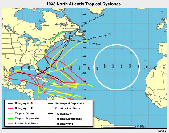
| Climatology | 2004 | 2005 | 1933 | |
| Named storms | 10 | 16 | 28 | 21 |
| Tropical Storms | 4 | 5 | 12 | 11 |
| Hurricanes | 6 | 9 | 15 | 10 |
| Subtropical storms | 1–2 | 1 | 1 | 0 |
8.7 Tropical Cyclone Motion
For over a century we have known that a tropical cyclone will move in response to the other weather systems in its environment.202,203 This view of tropical cyclone motion pictures it as a passive "cork in a stream" being "steered" by the other weather systems around it. Certainly, environmental steering (advection) is the dominant contribution to tropical cyclone motion. Advection of the storm by its environment can be approximated by the average wind through a deep layer of the atmosphere (the deep-layer mean wind).204,205,206 When calculating this wind from standard pressure level data, it is necessary to weight each level by the mass of the layer it represents. For tropical cyclone motion, the average from 850–200 hPa is used most often, however the choice of the averaging layer for the advection has been shown to be weakly related to storm intensity207 with a shallower (say 850–500 hPa) layer often estimating the steering better for weaker storms. While advection is clearly important, the limited success of forecasts using this approach led scientists to consider other mechanisms that also contribute to the motion of a tropical storm.
The most straightforward approach to the study of storm motion is to consider the motion due to the flow averaged through a deep layer, so we begin this study with the barotropic, nondivergent potential vorticity equation. The barotropic constraint means that we assume that the atmosphere has the same horizontal structure at all levels in the vertical, so it can be represented by the deep layer mean flow. Hence, the barotropic PV reduces to the vertical component of the absolute vorticity  .
.
The barotropic, nondivergent potential vorticity (PV) equation is written
 (9)
(9)where the variables have their usual meaning (given in Appendix A and Box 3-1 ). Equation (9) means that the absolute vorticity is conserved following the flow. So the relative vorticity,  , at a fixed location on the earth changes in time,
  , due to advection of absolute vorticity,
  .
.
where the variables have their usual meaning (given in Appendix A and Box 3-1 ). Equation (9) means that the absolute vorticity is conserved following the flow. So the relative vorticity, , at a fixed location on the earth changes in time, , due to advection of absolute vorticity, .
Scale analysis of Equation (9)208 shows that the most important term is the advection of relative vorticity, . However, observations show that if advection of Earth vorticity,
  , is not considered, an error in the motion of a few meters per second with a direction offset from the steering will occur. This error adds up in the course of a 24-hour or longer forecast. So we must consider this term, , which is known as the β–effect because β is the north-south variation of the Coriolis parameter.
 (10)
(10)8.7 Tropical Cyclone Motion »
8.7.1 The "β-Effect" and Environmental "β" effect
In addition to vortex motion due to steering by the large-scale flow, there is a contribution to tropical cyclone motion resulting from vortex interaction with the Earth's background vorticity gradient,208,209 known as either the β-effectk or as propagation due to the β-gyres. This vortex propagation component of the motion is typically smaller than the steering (often only a couple of m s-1 forward speed), but its impact on the storm direction can sometimes have substantial impacts on the storm evolution. This is because the change in direction can result in the storm interacting with different phenomena (other weather systems, SST anomalies, etc.).
In thinking about how the observed motion of a tropical cyclone differs from the motion expected if it were just blown along by the other weather features around it, we must understand the β-gyres.l Many authors give a straightforward mathematical analysis to demonstrate the physics of the formation of the β-gyres and their impact on tropical cyclone motion; a brief summary of these results is given here:
- Propagation (motion that is not advection) of a tropical cyclone could not occur without the north–south variation in the Coriolis parameter.
- The rotating winds of a tropical cyclone, combined with the north–south variation in the Coriolis parameter, induce relative vorticity asymmetries in the tropical cyclone (Fig. 8.60). These asymmetries are called the β–gyres.
- Since relative vorticity is calculated by taking spatial gradients of the vector wind, changes in vorticity must result in changes in the winds. Hence, the β–gyres must have winds associated with them.
- The winds of the β–gyres produce a net flow across the tropical cyclone center. Generally the β-drift is towards the northwest at a few knots; the speed and actual direction is related to the vortex size and strength.210
- In computer modeling studies, the β–gyres initially form at the radius of maximum winds (RMAX) of the tropical cyclone and are oriented so that the cyclonic β–gyre is to due east of the storm center and the anticyclonic β–gyre is to the west. This is true in both hemispheres.
- As the computer simulation evolves, the β–gyres move further out from the storm center and are rotated cyclonically by the storm's rotational winds.
- This final location and orientation of the β-gyres results in associated winds that cause the tropical cyclone to propagate poleward and westward in both hemispheres.
- In the real atmosphere we cannot see the β-gyres evolve in this way. In reality, development of the β-gyres occurs along with the evolution of the tropical cyclone and its environment.
Since we know that the tropical cyclone environment varies in the horizontal and vertical, it is important to study motion in the presence of more realistic environmental flows. The environmental vorticity gradients will change the structure of the β–gyres and so will change the propagation of the tropical cyclone compared to the steering.

The simple barotropic dynamics introduced here can still be used to understand the evolution of the "environmental β–gyres" for environments that have little variation in the vertical.177,211,212,213 Changes to the β–gyres due to a north-south environmental relative vorticity gradient are illustrated in Fig. 8.61.

k Interestingly, the Earth's vorticity gradient can be regarded as representing a second vortex of much larger scale than the tropical cyclone. In this way, the results in this section can be extended to both a synoptic-scale environment and to the Fujiwhara interaction of two or more tropical cyclones.
l These arguments are very similar to the conceptual model for the evolution of Rossby waves. Indeed, Rossby wave dispersion has been used to explain β–gyre evolution but the traditional treatment of Rossby waves considers a purely zonal background flow that results in westward propagation. It is the feedback of the vortex that provides the additional, poleward motion here.
8.7 Tropical Cyclone Motion »
8.7.2 Interaction of Vortices: The Fujiwhara Effect
For over a century it has been known that vortices will move in response to other vortices, even in an otherwise quiescent environment.202,203 Dynamically, this is just steering and environmental β–effect of one vortex on the other. Observational studies40,214 of the western North Pacific and North Atlantic document binary storm interactions on average 1.5 times per year for the western North Pacific and once every three years214 in the North Atlantic (for the period 1945-1981). Binary interactions occurred when the tropical cyclone centers were separated by distances of less than 1300 1400 km, but this critical separation distance depending on the sizes of the interacting systems.40,215 Of these interacting cyclones, 70% orbited cyclonically around one another with slower speeds of rotation around the other vortex with larger separation distance. The observed tropical cyclone motion is the combination of this rotation around the other vortex and any other environmental steering. The rotation of the two tropical cyclones around each other can be visualized by subtracting the average motion of the two storms from the motion of each storm separately (Fig. 8.62).
A comprehensive analysis of ten cases of tropical cyclone interaction provided a framework for discussion of binary storm interactions.216 By considering the centroid-relative track of the vortex pair, the storm-storm interactions can be separated into four components: (i) Approach and Capture, (ii) Mutual Orbit, (iii) Merger, and (iv) Escape (Fig. 8.62).
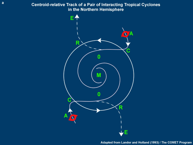
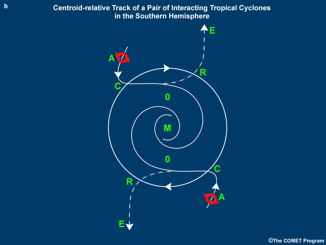
8.7 Tropical Cyclone Motion »
8.7.3 Other Factors Impacting Tropical Cyclone Motion
In our discussion of tropical cyclone structure, we explored a number of measures describing the radial structure of the rotational wind field (Fig. 8.13).33 These are the (1) intensity (peak surface winds), (2) strength (the average winds in an annulus outside the eyewall), and (3) size.
Strength is a measure of the variation of the rotational wind with radius: the shape of the profile. Intuitively, you know that a storm whose intense winds extend out a very large distance will be more damaging than a storm in which these winds drop off rapidly. These intense winds correspond to larger inertial stability (Section 8.2.3.2), and hence to a tropical cyclone that is more resilient to environmental influences.99 In extreme cases such as Supertyphoon Tip in 1979 (Box 8-3),27 this can mean that the storm generates its own steering flow and its motion is not dominated by surrounding weather systems. However, these situations are extremely rare. More commonly, the increase in inertial stability that follows from increased intensity minimizes the impact of strong vertical or horizontal wind shear on the storm.
Strength is a measure of the variation of the rotational wind with radius: the shape of the profile. Intuitively, you know that a storm whose intense winds extend out a very large distance will be more damaging than a storm in which these winds drop off rapidly. These intense winds correspond to larger inertial stability (Section 8.2.3.2), and hence to a tropical cyclone that is more resilient to environmental influences.99 In extreme cases such as Supertyphoon Tip in 1979 (Box 8-3),27 this can mean that the storm generates its own steering flow and its motion is not dominated by surrounding weather systems. However, these situations are extremely rare. More commonly, the increase in inertial stability that follows from increased intensity minimizes the impact of strong vertical or horizontal wind shear on the storm.
The relationship between the tropical cyclone motion and strength is generally closest when strength is evaluated between 3–5 degrees latitude radius (so approximately 300–500 km).206,207 Indeed, tropical cyclone propagation speed increases and its direction210 has a more westward component for increasing storm strength. The size of a tropical cyclone also relates to its propagation speed, but not its direction of propagation: larger tropical cyclones have a larger propagation speed than smaller storms.98,210,217,218
So more intense storms must also move more quickly—right? NO! Storm intensity is only weakly, and indirectly, related to its motion. One study of tropical cyclones in the Australian region has demonstrated that tropical cyclone intensity is linked to the layer over which the environmental winds advect the storm,207 but no significant link has been drawn between propagation and tropical cyclone intensity.210
Finally, vertical variation of both the tropical cyclone and its environment mean that its motion is not strictly that expected from barotropic dynamics. Vertical wind shear can affect the distribution of convection in the tropical cyclone. This can feed back onto the storm structure and so to the storm motion.
In summary, a tropical cyclone moves through a combination of advection by the average tropospheric winds of its environment and propagation due to the vorticity gradients of the Earth and its environment (including other tropical cyclones in Fujiwhara interactions), as well as variations in motion due to horizontal and vertical wind shear. The structure of the tropical cyclone (its size and inertial stability) will impact how the storm responds to all of these contributors to its motion: larger storms will have a larger propagation component of their motion; stronger storms will have a larger deviation between the direction of the advection and their motion; and the choice of the depth of the troposphere needed to calculate the environmental advection of the storm is weakly related to the storm intensity.
8.8 Societal and Environmental Impacts
Tropical cyclones are the most hazardous tropical weather systems. Their hazards include: strong winds, storm surge, wind-driven waves, heavy rainfall and flooding, tornadoes, and lightning.219,220,221 The impact of tropical cyclones can be categorized as direct and indirect or secondary impact.222 Direct impacts include coastal erosion by storm surge and loss of infrastructure from wind stress. Examples of indirect impacts are diseases associated with water contamination, oil price increases when drilling platforms and refineries are damaged or closed, and fires started by live, downed power lines. Economic loss from damage to crops and fisheries where livelihoods are dependent on agriculture, post disaster stress,40 and insurance rate increases are long term indirect effects. TCs remain a serious threat to society, especially as coastal population growth accelerates—a continuing trend in many locations around the world.137
8.8 Societal and Environmental Impacts »
8.8.1 Storm Surge and Wind-driven Waves
“The available documentation indicates that whenever there was a large loss of life from tropical cyclones, the predominant cause of death was drowning, not wind or windblown objects or structural failures.” Rappaport and Fernandez–Partagas (1995)
Globally, storm surge is the most deadly direct TC hazard.220,223 A storm surge is a large dome of water, 50 to 100 miles wide, that sweeps across the coast near where a hurricane makes landfall. It can be more than 15 feet deep at its peak (Fig. 8.63). The highest recorded death toll from a tropical cyclone occurred in November 1970; more than 300,000 persons were killed by coastal flooding when a cyclone made landfall in Bangladesh (Box 8-10).
Globally, storm surge is the most deadly direct TC hazard.220,223 A storm surge is a large dome of water, 50 to 100 miles wide, that sweeps across the coast near where a hurricane makes landfall. It can be more than 15 feet deep at its peak (Fig. 8.63). The highest recorded death toll from a tropical cyclone occurred in November 1970; more than 300,000 persons were killed by coastal flooding when a cyclone made landfall in Bangladesh (Box 8-10).
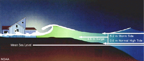
The storm surge is created by wind-driven waves with a very small component due to the low-pressure at the center of the cyclone. The surge is strongest where the winds are enhanced by the motion of the cyclone, therefore, the right (left) forward quadrant of the storm is the most dangerous storm surge region. While the waves may be relatively low in the open ocean, they gain height as they approach the coast (Fig. 8.63). The surge can move coastal structures and soil several miles inland. Geological studies have revealed layers of sediment in an Alabama lakebed believed to have been brought inland by storm surges as many as 3000 years ago.224 Storm surges are aggravated by high tide. Coastal flood models, such as the SLOSH model, are used to predict the storm surge.
Extratropical transition of tropical cyclones (Section 8.5) can cause extreme waves. For example, waves of over 30 meters were generated during the ET of Hurricane Luis (1995) causing extensive damage to the Queen Elizabeth II ocean liner. The extreme waves arrived only shortly before the main center of the storm. The growth of these waves have been explained in terms of "trapped fetch" in which the rapid forward motion means that the storm moves for a long time with the fastest growing waves123 (Fig. 8.64). As a result, waves generated during ET can be much larger than the waves generated by a TC. Enhancement in wave growth occurs only in the fastest wind region of the ET storm (where the storm winds and its forward motion are additive).
Extratropical transition of tropical cyclones (Section 8.5) can cause extreme waves. For example, waves of over 30 meters were generated during the ET of Hurricane Luis (1995) causing extensive damage to the Queen Elizabeth II ocean liner. The extreme waves arrived only shortly before the main center of the storm. The growth of these waves have been explained in terms of "trapped fetch" in which the rapid forward motion means that the storm moves for a long time with the fastest growing waves123 (Fig. 8.64). As a result, waves generated during ET can be much larger than the waves generated by a TC. Enhancement in wave growth occurs only in the fastest wind region of the ET storm (where the storm winds and its forward motion are additive).
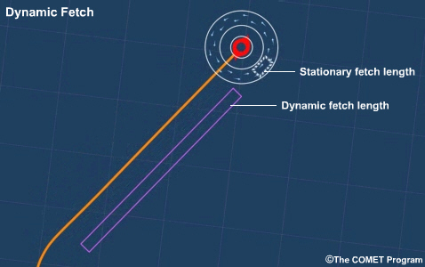
http://www.meted.ucar.edu/marine/mod2_wlc_gen/dynamic_fetch.htm
8.8 Societal and Environmental Impacts »
Box 8-10 The Deadliest Storms on Record: The Bangladesh Cyclones of 1970 and 1991
Disaster in 1970, The Bhola Cyclone
Imagine waking up to hear that over 300,000 – and possibly as many as 500,000 – of your countrymen had died. This really happened, and it was not hundreds of years ago. This unfathomable disaster happened on 12 November 1970 when the storm now known as the Bhola Cyclone made landfall in Bangladesh!
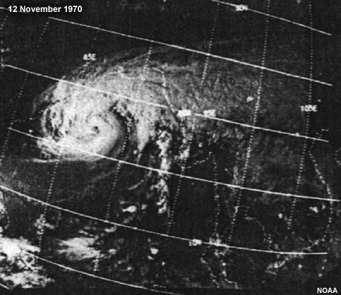
That night of 12 November 1970 the storm made landfall on the coast of East Pakistan (now Bangladesh). Many of the offshore islands were devastated by storm surge. The city of Tazumuddin (in the Bhola district of Bangladesh) was the most severely affected, with over 45% of the population of 167,000 killed by the storm. Topographic enhancement of rainfall by the mountains and storm surge make a devastating and deadly combination in the low–lying areas in the northern reaches of the Bay of Bengal.
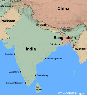
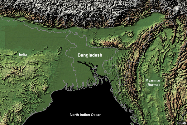
Disaster in 1991, the Chittagong Cyclone
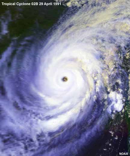
Tropical Cyclone 02B made landfall in Chittagong, Bangladesh on 29 April 1991 at about 1900 UTC. The official death toll from this storm was 138,000 people. Estimated damage was in excess of US $1.5 billion (in 1991 dollars). The coastal region was devastated by peak 1–minute averaged surface winds in excess of 72 m s-1 (260 km h-1), 898 hPa minimum pressure (Saffir–Simpson Category 5), and a 6.1 meter storm surge. However, as the 1970 Bhola storm demonstrated, the death toll could have been much higher. Evacuations of 2–3 million coastal residents were effective in reducing the fatalities, although the storm was still the largest natural disaster globally in 1991. The value of evacuation and shelter was demonstrated even more dramatically when powerful Category 4 Cyclone Sidr made landfall on 15 November 2007. The death toll was estimated at just over 3000 persons compared with the hundreds of thousands from the past cyclones. Although the damage was still costly and the destruction affected approximately 8.9 million people, better planning reduced fatalities by two orders of magnitude.225
Relative success in Bangladesh stands in contrast to tremendous loss of life in Burma (Myanmar) due to storm surge and flooding from Cyclone Nargis, May 2008. As of 21 July official death toll stood at 84,530; unofficial estimates were considerably higher.
http://www.reliefweb.int/rw/rwb.nsf/db900SID/ONIN–7GRR3J?OpenDocument&rc=3&cc=mmr
Indian Ocean Tropical Cyclone News,
http://www.scidev.net/en/agriculture-and-environment/tropical-cyclones-1/
8.8 Societal and Environmental Impacts »
8.8.2 Flooding and Landslides
Tropical cyclones are among the more prolific rainfall producers and the land surface response to heavy rainfall is one of the deadliest aspects of tropical cyclones. TCs rainfall produces flash floods, river floods, urban floods, and landslides. One of the deadliest hurricanes in the past decade was Mitch (1998), which killed more than 10,000 people when a week of rain caused landslides that covered entire villages (Box 8–4).
Tropical cyclones are among the more prolific rainfall producers and the land surface response to heavy rainfall is one of the deadliest aspects of tropical cyclones. TCs rainfall produces flash floods, river floods, urban floods, and landslides. One of the deadliest hurricanes in the past decade was Mitch (1998), which killed more than 10,000 people when a week of rain caused landslides that covered entire villages (Box 8–4).
Major flooding is not limited to hurricanes. Weak tropical storms can cause deaths and catastrophic damage. Recent examples include Tropical Storm Allison (2001) which produced more than 915 mm (36 inches) of rainfall over five days, caused 22 deaths, damage to over 48,000 homes, and exceeded $5.15 billion dollars in total damage in Texas and neighboring states.
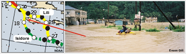
The amount, extent, and impact of TC flooding depend on the following:
- Antecedent precipitation: Saturated soil has greater flood potential than dry soil. An example of this is the case of Jamaica in 2002. The island received heavy rainfall as the eye of Tropical Storm Isidore passed to the south, 17-24 September. Only three days later, Tropical Storm Lili passed to the north and brought more heavy rain from 27-30 September (Fig. 8.65). From the two storms many rainfall records were broken; many places received more than 600% of their September normal rainfall. Another example is Central America, where Mitch (1998) struck near the end of the rainy season when soil was saturated.
- Speed of movement of the cyclone: Slower movement leads to greater flooding.
- Orographic enhancement: Additional lifting of moist air by high terrain produces more precipitation.
- Intensification due to synoptic forcing: Interaction of the cyclone with midlatitude synoptic systems can sometimes enhance the low pressure and increase precipitation. A prime example is Hurricane Agnes (1972), which interacted with a midlatitude trough and produced widespread river flooding in the northeastern US (Fig. 8.66). Property loss from the inland flooding of Agnes was $3.5 billion dollars compared with $10 million of losses from its landfall in Florida.
- Hydrology: Narrow river basins are easier to flood than flat, broad river basins. Confluence of multiple rivers can also aggravate flooding. Bangladesh is one of the most vulnerable places for flooding because it is the confluence of major rivers and at the mouth of the Bay of Bengal.
- Land use: Urban landscapes are more prone to flash floods because of increased runoff and channeling which causes acceleration of surface water. Denuded hillsides are more prone to landslides; plant roots help to stabilize the soil.
- Other geographical influences: Flooding is also influenced by soil type. Soils with slow infiltration lead to greater runoff and flooding.
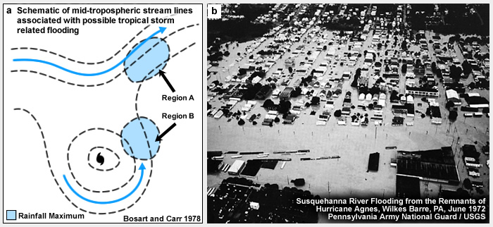
8.8 Societal and Environmental Impacts »
8.8.3 Strong Winds and Tornadoes
The wind velocity is a defining parameter for TCs because of the deadly and damaging impact of strong winds (Fig. 8.67). The Saffir Scale was created to provide guidance on the effects of strong winds (Box 8-3).
The wind velocity is a defining parameter for TCs because of the deadly and damaging impact of strong winds (Fig. 8.69). The Saffir Scale was created to provide guidance on the effects of strong winds (Box 8-3).
In addition to the strong winds associated with the landfalling tropical cyclone, extremely strong winds are generated in tornadoes that sometimes also accompany a TC. As a tropical cyclone makes landfall, the surface winds decrease faster than winds above, creating vertical wind shear which allows for tornadoes to develop. Most tornadoes develop in the right-forward (left-forward) quadrant of the cyclone in the northern (southern) hemisphere. Most tornadoes are reported in the outer rainbands226 where vertical wind shear is favorable. Tornadoes in the intense inner core are produced by eyewall mesovortices.227
In the US, hurricanes recurving to the northeast were more likely to produce tornadoes than those moving westward, possibly due to enhancement of low-level shear from a 500 hPa trough.228
8.8 Societal and Environmental Impacts »
8.8.4 Lightning
Lightning in TCs is a small percentage of total global lightning. When lightning does occur in TCs, it most often happens in the convective outer rainbands.229,230,231 The highest density of flashes is frequently on the eastern side of storms (e.g., Fig. 8.68).
8.8 Societal and Environmental Impacts »
8.8.5 Impacts of Extratropical Transition
As discussed in Section 8.5, tropical cyclones undergoing ET may initially weaken as they move into the extratropics, but they can reintensify into midlatitude storms that are occasionally more intense than their tropical selves (e.g. Hurricane Irene in 1999), often traveling at forward speeds of 15–20 m s-1. These intense weather phenomena can exist long after their "tropical storm" status has been discontinued. The remnant tropical storm can also provide a source of enhanced thermal contrast for the later development of an intense midlatitude storm. The rapid forward speed, large area of gale force winds, intense asymmetric precipitation zone, and potential for extreme ocean waves associated with ET events (Section 8.8.1) make these challenging systems to forecast.
As discussed in Section 8.5, tropical cyclones undergoing ET may initially weaken as they move into the extratropics, but they can reintensify into midlatitude storms that are occasionally more intense than their tropical selves (e.g. Hurricane Irene in 1999), often traveling at forward speeds of 15–20 m s-1. These intense weather phenomena can exist long after their "tropical storm" status has been discontinued. The remnant tropical storm can also provide a source of enhanced thermal contrast for the later development of an intense midlatitude storm. The rapid forward speed, large area of gale force winds, intense asymmetric precipitation zone, and potential for extreme ocean waves associated with ET events (Section 8.8.1) make these challenging systems to forecast.
The changing structure of the ET system compared to its "parent" tropical cyclone means that the area of damaging winds is much larger and typically confined to the right (left) of a NH (SH) cyclone looking towards its direction of motion. The rain region is also larger and is located on the opposite side to the strongest winds.
8.8 Societal and Environmental Impacts »
8.8.6 Hazard Mitigation
Catastrophes such as the Bangladesh cyclones, TC Nargis, and Hurricane Katrina highlight the need for mitigation measures that take into consideration both the physical and social aspects of tropical cyclones. Hazard mitigation is multi–faceted, involving long–term planning (education, building codes and zoning) and short term planning (responding to an individual event and its immediate aftermath). Mitigation against tropical cyclone impacts includes improvements in TC forecasting, understanding the sources and distribution of societal vulnerability, understanding the long–term impact of coastal environmental change (e.g., removal of marshes), up-to-date floodplain maps, land use planning and building codes, warning systems tailored to reach all populations. One of the challenges of mitigation for tropical cyclones is that the responsibilities for the various aspects (warnings, education, zoning, recovery, etc.) are spread across a range of levels and departments of government, varying by country and region; no single tropical cyclone strategy operates.
The success of TC hazard mitigation by public education on the dangers of storm surge was demonstrated during the landfall of Cyclone Sidr in Bangladesh on 15 November 2007. Cyclone Sidr was a category–4 cyclone, yet deaths numbered a few thousands232 instead of the hundreds of thousands during past cyclones of similar magnitude. Unfortunately, mitigation against deaths from storm surge remains uneven around the Bay of Bengal, as demonstrated by the tremendous loss of life when Tropical Cyclone Nargis made landfall in Burma (Myanmar) on 2 May 2008 (Box 8–10). In the US, public education on inland flooding was jumpstarted when it was reported that freshwater flooding from tropical cyclones was the largest single cause of hurricane-related deaths in the United States between 1970 and 1999.233
The success of TC hazard mitigation by public education on the dangers of storm surge was demonstrated during the landfall of Cyclone Sidr in Bangladesh on 15 November 2007. Cyclone Sidr was a category–4 cyclone, yet deaths numbered a few thousands232 instead of the hundreds of thousands during past cyclones of similar magnitude. Unfortunately, mitigation against deaths from storm surge remains uneven around the Bay of Bengal, as demonstrated by the tremendous loss of life when Tropical Cyclone Nargis made landfall in Burma (Myanmar) on 2 May 2008 (Box 8–10). In the US, public education on inland flooding was jumpstarted when it was reported that freshwater flooding from tropical cyclones was the largest single cause of hurricane-related deaths in the United States between 1970 and 1999.233
Timely evacuation from storm surge has been successful in reducing loss of life from tropical cyclones. However, evacuation is a complex issue for officials and the general population. Can you think of some issues that need to be considered? For example, think of situations in which evacuation may not be possible or advisable.
(Type your answer in box.)
Feedback:
Issues associated with evacuation include, but are not limited to the following: On small islands, residents must shelter in place, unlike continental regions where coastal residents can move far inland. Evacuation is costly and the cost will not be replaced if there is no impact. It is not advisable to evacuate when the evacuation time is longer than the forecast lead time or when the evacuation route is impassable. Maps of evacuation boundaries often do not recognize the difference between discomfort (standing, shallow water) and deadly harm (moving water and drowning). Assessment of those differences could reduce the number of unnecessary evacuees. Uncertainty in the forecast makes evacuation decisions more difficult.
Warning and evacuation declarations are the mitigation strategies employed immediately prior to a tropical cyclone impacting a location. Effective warning systems require the integration of monitoring technology, evacuation plans and procedures, and personnel. Sorensen (2000)234 reviewed twenty years of warning systems and found several major factors that affect the desired response to a warning or evacuation declaration. Response was most affected by physical cues (e.g., images of the size and intensity of the storm); proximity to the threat; experience with hazards,m and social cues (e.g., trusted neighbors evacuating). It should be understood that mitigation is a continuous process of adjustment and improvement.
UN Report, TC Sidr,
http://www.reliefweb.int/rw/dbc.nsf/doc108?OpenForm&rc=3&emid=TC-2007-000208-BGD
NASA, TC Nargis,
http://www.nasa.gov/mission_pages/hurricanes/archives/2008/h2008_nargis.html
UN Report, TC Nargis,
http://www.reliefweb.int/rw/rwb.nsf/db900SID/ONIN-7GRR3J?OpenDocument&rc=3&cc=mmr
WMO Links to Active National Warnings of Tropical Cyclones,
http://www.wmo.int/pages/prog/www/tcp/National%20Warnings.html
United Nations Stop Disasters game, http://www.stopdisastersgame.org/en/
m For example, experience with Hurricane Camille led some coastal residents to flee from Hurricane Katrina while others stayed because they had survived Camille.
Focus Areas
Focus Areas »
Focus List
Focus 1: Tropical Cyclone Ingrid (2005)
Focus 2: The Most Intense Tropical Cyclones
Focus 3: Hurricane Mitch (1988): Devastation in Central America
Focus 4: Rare South Atlantic Tropical Cyclone Catarina (2004)
Focus 5: Severe Tropical Cyclone Gonu (2007)
Focus 6: Unusually Active Seasons around the Globe
Focus 7: The Deadliest Storms on Record
Focus Areas »
Operational Focus
Why we forecast tropical cyclones
Global Distribution and Monitoring of Tropical Cyclones (TC)
- Classification of Tropical Cyclone Intensity around the World
- Monitoring of Tropical Cyclones, WMO Regional Centers
Tropical Cyclone Structure
Tropical Cyclogenesis
- Necessary conditions for tropical cyclone formation
- Genesis in the monsoon trough, schematic of TC formation region
- TC formation and Tropical Upper Tropospheric Troughs (TUTT)
- TC formation and Equatorial Waves
- TC formation and African Easterly Waves
- TC formation from subtropical storms or “Tropical Transition”
- Mesoscale Influences on TC formation
- Global maps of tropical cyclogenesis sources and modulating influences
Will the Tropical Cyclone Vortex survive?
Tropical Cyclone Intensity
- Lifecycle of Tropical Cyclones, Example of Rita (2005),
- Dvorak Technique, Satellite Estimate of TC Intensity
- Why is it that every storm is not a Cat. 5?
- Eyewall replacement cycles and TC intensity
- TC Intensity and radius of 34-kt wind
- Inner core features and links to intensity
Satellite and Radar Remote Sensing of Tropical Cyclones
- Observing 3-D structure from remote sensing
- Dvorak enhanced IR technique for estimating intensity
- Satellite microwave analysis of TCs
- Parallax error in locating the eye
- Eyewall replacement cycles and TC intensity
- Satellite-derived Winds
Climatology of Tropical Cyclones
- Seasonality of TC formation
- Intraseasonal or sub-seasonal influences on TC occurrence
- Seasonal Forecasting of TC Activity
- Interannual Variability
Tropical Cyclone Motion
- The Beta-Effect or Why tropical cyclones move westward and poleward even without steering flow
- How tropical cyclones move relative to each other, the Fujiwhara Effect
Extratropical Transition
Tropical Cyclone Impacts
- Video of landfalling TC Ingrid (2005)
- Storm surge and Wind Driven Waves
- Flooding and landslides
- Post-landfall structural changes
- Strong Winds and Tornadoes
- Lightning
Tropical Cyclone Hazard Mitigation
Summary
Tropical cyclones affect around half of the globe and more than half of the Earth's population. Familiarity with the necessary large-scale environmental conditions for tropical cyclogenesis helps explain the distribution of these storms around the world. Understanding of both extratropical and tropical transitions provides insights into the sources of tropical storm activity in other regions. Theories for potential intensity (PI) give guidance on likely tropical cyclone peak intensity, but the effects of environmental factors ensure that very few tropical cyclones achieve their PI. Their three-dimensional rotational wind distribution results in inertially stable, warm-cored vortices. This inertial stability provides some insulation for the tropical cyclone from environmental forcings; however weak tropical cyclones and the upper tropospheric outflow region of all storms are less protected by inertial stability. The societal impacts of tropical cyclones can be devastating and widespread, inspiring our attention and further studies of the atmosphere.
Appendix A: List of Principal Symbols
| θe | Equivalent potential temperature (K) |
|
Rossby number (non-dimensional) |
| V | scale wind speed (m s-1) |
| L | scale length (m) |
| f = 2Ω sin(φ) | vertical component of the Coriolis parameter (s-1) |
| Ω | Earth rotation rate = 7.292×10⁻⁵ (s-1) |
| φ | latitude (radians) |
 |
latitudinal gradient of the Coriolis parameter (s-1 m-1) |
| a | radius of the Earth = 6.37×10⁶ (m) |
| fo | reference value of Coriolis parameter, f, at latitude φo (s-1) |
| I2=(ζ+fo)(fo+v/r) | inertial stability |
| ζ | vertical component of relative vorticity |
| v | rotational wind speed |
| r | radius |
 |
thermal wind |
 |
geostrophic wind |
| pA | pressure above |
| pB | pressure below |
| R | Universal gas constant = 287 J kg-1 K-1 |
| g | gravity (m s-2) |
| B | CPS parameter (thermal asymmetry) |
| VTL | CPS parameter (lower tropospheric thermal wind) |
| VTU | CPS parameter (upper tropospheric thermal wind) |
 |
Rossby radius of deformation (m) |
| (u, v) | symmetric averages of the cylindrical wind components |
| (u', v') | asymmetric components of the cylindrical wind |
|
saturation equivalent potential temperature |
 |
specific absolute angular momentum (m2 s-1) |
 |
vector radius from the Earth axis of rotation |
| r | distance from the Earth axis for this application (m) |
 |
absolute velocity (Earth motion plus wind) (m s-1) |
 |
vertical component of the absolute vorticity (s-1) |
 |
Lagrangian (total) derivative ("following the flow") |
 |
Eulerian derivative (at a fixed location) |
 |
advection of the vertical component of absolute vorticity |
 |
total wind partitioned into symmetric and asymmetric components |
 |
total wind partitioned into symmetric, environment, gyres |
Questions for Review
- Identify five parts of the tropical cyclone and where you would expect to find them with respect to the surface center of the storm.
- List six necessary, but not sufficient, conditions that must be present in the large scale environment for tropical cyclogenesis to occur.
- Summarize the six conditions you have just listed into two physical constraints necessary to achieve genesis.
- Discuss the tropical cyclone mean spatial and seasonal distribution (global climatology) with reference to these "necessary but not sufficient conditions."
- Identify (a) two intraseasonal and (b) two interannual or interdecadal phenomena that modulate tropical cyclone activity. In the context of the "necessary but not sufficient conditions for genesis, discuss how one phenomena from each of (a) and (b) leads to variations from the mean tropical cyclone climatology.
- Identify four potential incipient disturbances that could lead to tropical cyclogenesis.
- Can tropical cyclogenesis occur without an incipient disturbance? Discuss.
- Identify and describe the six possible stages of a tropical cyclone lifecycle. Two of these stages may not occur in an individual tropical cyclone lifecycle—which ones?
- Using satellite remote sensing techniques, describe how you could detect changes in the intensity and structure of tropical cyclones.
- Describe the process of evolution from an incipient tropical disturbance to an intense tropical cyclone.
- How does evolution from a subtropical cyclone (tropical transition) differ from the answer just given?
- Discuss how inner core dynamics can lead to changes in cyclone structure and intensity.
- Define potential intensity (PI).
- The two main theories for potential intensity are CISK and WISHE. What is the key distinction in the fundamental CISK and WISHE assumptions?
- Why does every tropical cyclone not become a severe tropical cyclone? Discuss with reference to both the PI theories and the climatological atmospheric flow patterns of the global tropics.
- What are the characteristics of tropical cyclones that undergo extratropical transition?
- What kind of environmental support is necessary for extratropical transition?
- Describe various mechanisms that lead to extratropical transition.
- Describe the mechanisms that influence tropical cyclone motion. Consider the impacts of the storm environment, including the presence of multiple storms.
- Describe the hazards of tropical cyclones particularly those at landfall (storm surge, heavy rain and floods, strong winds, tornadoes, ocean waves) and discuss the basic mechanisms for each type of hazard.
QUIZ
You may also take a quiz and email your results to your instructor.
Brief Biographies
Dr. William M. Gray
"He's still lanky, like the baseball player he used to be back at Woodrow Wilson High School in Washington in the 1940s. He's the guy who, every year, predicts the number of hurricanes that will form during the coming tropical storm season. He's mentored dozens of scientists." Washington Post (26 May 2006)
William M. (Bill) Gray is an Emeritus Professor of Atmospheric Science at Colorado State University. While hurricane enthusiasts in the wider community may recognize Dr Gray specifically for his seasonal hurricane forecasting, his scientific career has spanned all aspects of tropical cyclones from their genesis and motion to their climate variability. Through his adept use of the available observations, Professor Gray has shed insight on tropical cyclogenesis and climatology, the evolution of storm structure and intensity, and tropical cyclone motion. He has mentored numerous students and colleagues throughout his career of more than 40 years, further extending his impact on the field. Bill Gray's achievements have been widely recognized, including the Jule L. Charney and Banner I. Miller Awards of the American Meteorological Society.
Early in his career, Professor Gray served as a weather forecaster for the United States Air Force. He received his Ph.D. from the Department of Geophysical Sciences at the University of Chicago in 1964 and has served since 1961 on the Department of Atmospheric Science faculty at the Colorado State University. Bill Gray is a Fellow of the American Meteorological Society.
Dr. Kerry A. Emanuel
"Behold, a whirlwind of the Lord is gone forth in fury, even a grievous whirlwind: it shall fall grievously upon the head of the wicked." Jeremiah, 23:19.
And so begins The Divine Wind, Emanuel's comprehensive review of the history and scientific understanding of hurricanes. Kerry Emanuel is a Professor of Earth, Atmospheric and Planetary Sciences (Program in Atmospheres, Oceans, and Climate) at the Massachusetts Institute of Technology. Kerry received his doctorate from MIT in 1978, then joined the faculty of UCLA. After some years, Kerry returned to MIT, now as a member of its faculty.
Dr Emanuel's contributions to the understanding of tropical cyclones are broad and include the ongoing development, rigorous review and refinement of a theory for the potential peak intensity for tropical cyclones, mechanisms of scale selection in the tropics, tropical convection and climate change impacts on hurricanes. His theory of tropical cyclone potential intensity has provided a framework for considering the impacts of climate change on tropical cyclones. Kerry has mentored many young scientists; he is the author (or co-author) of more than 100 journal and review articles, as well as three books. Kerry Emanuel's honors and awards include the American Meteorological Society's Meisinger Award and Carl Gustaf Rossby Medal.